The University’s mail relays and encryption

By the time this post has been published, the Oxmail relays will most likely be using opportunistic encryption to encrypt outgoing emails, in response to actions by cloud mail providers. However, we would like to make it clear that we have always known that we had encryption disabled and that our reasons for enabling it have nothing to do with addressing privacy concerns. This post should hopefully explain all this along with some relevant history.

What is SMTP?

Simple Mail Transport Protocol is the de-facto standard for email transfer between servers. SMTP is an old standard and at its inception the internet was a happier place with less need for security and thus no security was built into the protocol. Mail delivery is via a hop by hop mechanism, which is to say that if I fire off an email to fred.bloggs@example.org, my mail client does not necessarily contact Fred’s mailstore directly, rather it contacts a server it thinks is better suited to deliver the mail to Fred. It is a very similar concept to 6 degrees of separation. The Oxmail relays are one hop in the chain from the sender, you at your laptop (other devices are available), and the destination server which houses the mailbox of Fred Bloggs.

This is just an example of the many servers that need to participate to get an email from your laptop to a recipient.

This is just an example of the many servers that need to participate to get an email from your laptop to a recipient. The number of servers is variable and you do not necessarily know the number when sending an email.


What is TLS?

TLS, or Transport Layer Security to give its full name, is a mechanism by which each hop is encrypted so that eavesdroppers in the middle of the connection cannot listen in on the transfer. To be clear, routers and most firewalls are not considered endpoints in this context, it’s just the mail servers that are set up to route mail to particular destinations, and as such these routers and firewalls are exactly the devices for which this mechanism is designed to protect against.

Why did the Oxmails not encrypt mail?

I should start by saying that there was nothing inherently stopping the Oxmail relays from initiating an encrypted communication when sending mail. The software that we run is capable of encrypting communications, and in fact we require it for incoming external connections to smtp.ox.ac.uk, so as to protect password credentials from being harvested. However, we have reservations with the concept of TLS encryption for a few reasons:

  • Since SMTP is a hop-by-hop protocol with an email traversing multiple servers A through to G, just because the communication between F and G is secure you know absolutely nothing about how secure your email is. For G to know that the email received is actually from A and is unaltered, every point needs to be encrypted, and yet there is no way of telling G that this is the case. All G knows is that the last hop was secure.
  • As almost a repetition of the last sentence, TLS does not necessarily make communications any safer and pretending otherwise is bordering deceitful. Similarly, if the mail received by G is set to be forwarded to another mailbox H, and this is done via an encrypted channel, is that now secure?
  • The battle may already be lost on this since its uptake is so small, but there is a technology that was designed to solve this: GPG. Using GPG, you encrypt the email using your laptop and only Fred can decrypt it, unlike TLS where each hop has access to every email’s contents. The truly security conscious should be using GPG to encrypt mail as only the recipient and sender can see the message. The necessary data to decrypt the message is stored locally on your computer.

To summarize these points, we did not encrypt outgoing mail as we considered it a pointless exercise that would only give people the illusion of security without actually doing anything.

Why are we now enabling opportunistic encryption on the Oxmail relays?

Following the actions of cloud service providers, where emails received unencrypted were flagged to the person reading the mail, we were presented with two options:

  • Do nothing.
  • Implement TLS.

The former may have been our stance, but recently we have been receiving complaints that sent emails’ privacy has been violated when sent to certain mail providers. Rather than argue the point that email as an entire concept is insecure (after all there is nothing stopping cloud mail providers from reading your emails for account profiling and targeted advertising), the change is relatively minor our end and so we took the conscious decision to enable outgoing TLS when available, so as to remove the flag on mail sent to these cloud providers.

Are there better solutions available?

Yes! Even better, some of these solutions can be used today without any change on any infrastructure (except perhaps your mail client). I mentioned GPG above which is completely compatible with the existing infrastructure used around the world. You could even post your emails onto a public share using a service such as Dropbox with a link to it on Twitter and still only the recipient can read it. I must admit that usage of GPG is minimal despite its relative maturity and perhaps going into the reasons is not beneficial to the current discussion. There is also an encryption mechanism called S/MIME which has the same overall effect as GPG, even though its method is quite different. S/MIME reportedly is better supported by more mail clients, but requires purchasing a digital certificate and is thus potentially more expensive than GPG [update: this is incorrect. They can be obtained free of charge. See comments].

Added to GPG and S/MIME there are SPF and DKIM which can help verify servers’ authenticities (they do not encrypt). These technologies themselves are not well suited to our (the University’s) devolved environment as outlined in an excellent blog post by my predecessor Guy Edwards.

Conclusion

I hope this helps explain our thoughts on TLS encryption, and that our recent change to use encrypted communications is not a reaction to a mistake we discovered we were making. If there is anything you wish to add, please do add a comment, or contact the IT Services helpdesk for further information.

Posted in Mail Relay, Message Submission | Tagged , , | 4 Comments

DNS Resolvers – DNSSEC

We are approaching deployment of a new fleet of DNS resolvers and there are a few questions that we would like feedback from the wider ITSS community. Specifically this post is broaching the subject of DNSSEC. Just to be clear, this is nothing to do with securing and signing our own zones (ox.ac.uk being but an example), but rather whether we will request and validate signed responses from zones who have already implemented DNSSEC. I have views and opinions on this matter, but I will put them to one side and offer an untainted exposition. If my bias creeps through then I apologize.

On the subject of comments, whereas I welcomed comments in my previous blog posts, I actively encourage it here. A dialogue would be nice in an informal channel and will hopefully help us reach a consensus. The informal place is because ultimately, you are free to do whatever you like with the validation data; this is only to decide the central resolvers’ default behaviour.

What is DNSSEC?

Hopefully you are already aware of what DNSSEC does, and possibly how it achieves it. There are some good guides already online explaining DNSSEC. In essence, before DNSSEC, you had to take it on trust that the reply you received for a DNS query was valid. In some sense, nothing has changed, you are still trusting that the DNS resolvers are correctly validating any responses received (by default, you are free to replicate the validation yourself). However, you can now be sure that if you want www.cam.ac.uk to resolve to an IP address, with DNSSEC requested (via something called an AD bit), any validated response will either be the correct answer, or will fail (NXDOMAIN).

Does this decision affect me?

I am running my own resolver / am not using the central resolvers
No
I’m running a stub resolver and am using the central resolvers as a forwarder
Potentially
I’m running a stub resolver and validating my own queries
No
I’m running a laptop plugged into eduroam and am using the DNS resolvers provided by DHCP
Potentially
I’m running a laptop connected to OWL and have authenticated as a guest
You shouldn’t be a member of the University and connected to OWL, but in any case no.

Why is it good?

This subheading is almost redundant as it should be fairly clear what the benefits of DNSSEC are. Any request for a record in a signed zone will always be relied upon to be correct (unless there has been a SIG key breach or some other disaster.) This means that problems in the past, like cache poisoning are just that; problems of the past. If you want to ensure that a hostname resolves to an IP address with confidence that no man-in-the-middle has tampered with any response, then there really is no other tool available, it’s DNSSEC or nothing.

Why is it not so good?

  1. There is additional complexity. For us to deploy resolvers that validate records, it’s just a simple configuration option. However, for those zones that are signed, the ease at which you can make every record you serve an NX (aka Not found) is alarming. Since I have worked here, one organization has gone completely dark to the outside for validating resolvers due to key mismatches, and another due to TTLs on expired keys. Any records would have resolved on any resolvers which didn’t do validation.
  2. Not every zone is signed. This really shouldn’t affect our decision since unsigned zones work fine whatever we decide, but there is the next point to consider
  3. Validating zones and records adds complexity to a resolver. We use BIND and the list of recent vulnerabilities shows that a not insignificant number of them are related to DNSSEC. Some have not affected us as we do not currently do any validation.
  4. Your opinion may vary on this, but most important information on the internet is signed by other means already. Windows and Linux updates are almost without exception signed by an organization (perhaps some viruses don’t) and websites employ SSL to secure web communication. If you are concerned with the efficacy of SSL in general, then conceptually DNSSEC is no different; if a zone is compromised, then it’s compromised in all the sub-zones.

I disagree with the decision of validating/not validating on the new resolvers! What can I do?

DNSSEC is supposed to be completely backwards compatible with existing infrastructure. I know of one unit that is validating all records while using the existing central resolvers as forwarders (as a point of information, it was this unit that led to the discovery of the TTL expiry NXDOMAIN problem. Most requests for this organization were being resolved fine as we weren’t validating!)

So, whatever the final outcome, there is nothing stopping anyone from running a STUB resolver that either asks to remove signing responsibility from the central resolvers (via the CD flag) or by requesting the extra DNSSEC records (via the DO flag). However, whatever is decided will be used for eduroam and unless you wish to configure individual clients, there will be no provision to change this.

Conclusion

In some sense, there is not yet any conclusion. If you wish to ask me to expand on any point, of if I have neglected anything, then please write a comment below. The benefits are obvious, but hopefully this article lists some concerns that should at least be acknowledged if we are to validate zones by default.

Updates

Following are reponses to emails received:

Could you elaborate on the potential issues for someone running a laptop plugged into eduroam and am using the DNS resolvers provided by DHCP – that would probably account for two-thirds or more of the folk here these days.

The potential issues are exactly the same as outlined above, but for users connected to eduroam. These are the problems of mismatched keys and BIND vulnerabilities resulting in outages.

Posted in DNS | 6 Comments

FreeRADIUS, sql_log, PostgreSQL and upserting

While this is superficially a post for creating an upsert PostgreSQL query for FreeRADIUS’s sql_log module, I felt the problem was general enough to warrant an explanation as to what CTEs can do. As such, the post should be of interest to both FreeRADIUS administrators and PostgreSQL users alike. If you’re solely in the latter camp, I’m afraid that knowledge of the FreeRADIUS modules and their uses is assumed, although the section you’ll be most interested in hopefully can be read in isolation.

The problem

All RADIUS accounting packets received by our RADIUS servers are logged to a database. Previously we used the rlm_sql module included with FreeRADIUS to achieve this, which writes to the database directly as a part of processing the authentication/accounting packet.

Here we can see that when a RADIUS packet arrives at the FreeRADIUS server, it is immediately logged in the database

When using rlm_sql, a RADIUS packet arrives at the FreeRADIUS server, it is immediately logged in the database.

However, we decided to change to using rlm_sql_log, (aka the sql_log module) which buffers queries to a file for processing later via a perl script.

rlm_sql_log buffers queries to a file before executing at a later date.

rlm_sql_log buffers queries to a file before executing at a later date.

At the expense of the database lagging real life by a few seconds, this decouples the database from the FreeRADIUS daemon completely and any downtime of the database will not affect the processing of RADIUS packets. Another benefit is that rlm_sql requires as many database handles (or database connections) as packets it is processing at any one time. For us that was 100 connections per server, which almost certainly would be inadequate now that our RADIUS servers are under heavier load. Using rlm_sql_log we now have one connection per server.

However, the rlm_sql module had a nice feature we used where update (eg. Alive, Stop) packets would cause an update of a row in the database but if the row didn’t exist one would be created. If you look at the shipped  configuration file for sql_log, you will see that this behaviour is not available as a configuration parameter and every packet results in a new row in the database, even if a previous packet for the same connection has already been logged. The reason that it chooses to do this is fairly obvious: there is no widely implemented SQL standard which defines a query that updates a row, and inserts a new one if it doesn’t exist. MySQL has its own “ON DUPLICATE KEY UPDATE…”, but we use PostgreSQL and even if we did use MySQL, such a mechanism would not work without modification to FreeRADIUS’s supplied schema.

One could in theory change the INSERT statements for UPDATE statements where appropriate (i.e. everything but the start packet), but bear in mind that RADIUS packets are UDP, and as such their delivery isn’t guaranteed. If the start packet is never received, then UPDATE statements will not log anything to the database.

The solution

Common Table Expressions

The IT Services United Crest

The IT Services United Crest

The SQL 1999 spec defined a type of expression called a Common Table Expression [CTE]. PostgreSQL has been able to use these expressions since 8.4 and, although not sold as such, they are a nice way of simulating conditional flow in a statement, by using subqueries to generate temporary tables which affect the outcome of a main query. Said another way, a simple INSERT or UPDATE statement’s scope is limited to a table. If you want to use one SQL query to affect and be based upon the state of multiple tables without using some kind of glue language like perl, this is the tool to reach for

The official documentation contains some examples, but I will include my own contrived one for completeness.

Say a professional football team existed, IT Services United. Each player for the purposes of this exercise has two interesting attributes, a name and a salary, which could potentially be based on the player’s ability. In a PostgreSQL database the table of players could look like the following:

          Table "blog.players"
 Column |       Type        | Modifiers 
--------+-------------------+-----------
 name   | character varying | not null
 salary | money             | not null
Indexes:
    "players_pkey" PRIMARY KEY, btree (name)
Check constraints:
    "players_salary_check" CHECK (salary > 0)

If you wanted to give everyone a 10% raise, that’s not too difficult:

UPDATE players SET salary = salary * 1.1;

So far so good. Now, as most people can attest I am not great at football, so everyone else on the team deserves a further raise as recompense.

UPDATE players SET salary = salary * 1.2 WHERE name != 'Christopher';

On the face of it this query should be sufficient. However there are deficiencies. I may not be playing for IT Services United (I may have recently signed for another team), in which case the raise is unjustified. Also this money has to come from somewhere. We should be taking this money out of my salary as this is being done as a direct consequence of my appalling skills on the pitch.

In summary we would like to do the following:

  1. Check to see if I’m a player, and do nothing if I’m not
  2. Find the sum of the salary increase for all players excluding me
  3. Deduct this sum from my salary
  4. Add this to each player accordingly

Doing this in one query is not looking so simple now. People normally faced with this scenario would use a glue language and multiple queries, but we are going to assume we do not have that luxury (as is the case when using rlm_sql_log).

There are other things to consider as well:

  • Rounding is an issue that cannot be ignored especially when it comes to money. For the purposes of this example the important number the total outgoing salary given to the team, SUM(salary), is constant but this would need much more scrutiny before I used this for my banking say.
  • The problem of negative salaries has already been taken care of as a table constraint (see the table schema above). If any part of the query fails, then the whole query fails and there is no change of state.

Here’s a query that I believe would work as billed:

WITH salaries AS (
 UPDATE players
  SET salary = players.salary * 1.2 -- ← Boost salary of the players

  FROM players p2           --  |Trick for getting
  WHERE                     -- ←|original salary
   players.name = p2.name   --  |into returning row

  AND       -- ↓ Check I'm playing ↓
   exists ( select 1 from players where name = 'Christopher') 

  AND
   players.name != 'Christopher' -- ← I don't deserve a raise

  RETURNING                       --  |RETURNING gives a SELECT like
   players.salary AS new_salary,  -- ←|ability, where you create
   p2.salary AS original_salary,  --  |a table of updated rows.
   players.salary - p2.salary AS salary_increase
)
  UPDATE players -- ↓ Deduct the amount from my salary ↓
   SET salary = salary  - (SELECT sum(salary_increase) FROM salaries)
   WHERE name = 'Christopher';

For people who dabble in SQL occasionally this query might seem a bit dense at first, but the statement can be made clearer if broken down into its components. Here are some that deserve closer scrutiny:

WITH salaries AS (………)
This is the opening and the main part of CTEs. It basically says “run the query in the brackets and create a temporary table called salaries with the result.” This table will be used later
UPDATE …… RETURNING ….
UPDATE statements by default only shows the number of rows affected. This is not much use here so adding “RETURNING ….” to the statement returns a table of the updated rows with the columns you supply in the statement. This becomes the salaries table.
UPDATE …. FROM ….
When using RETURNING, unfortunately you cannot return the values of the row prior to its update. However, you are allowed to join a table in an update statement using FROM. In this example we are using a self join to join a row to itself! When the row is updated the joined values are unaffected by the update and can be used to return the old values.
SET salary = salary – (SELECT sum(salary_increase) FROM salaries)
Each individual salary_increase is in the temporary table salaries, but we need the sum of these values. Because of this we need to use a subquery within the second update statement.

This example is so contrived as to be silly, but you can see how we have been able to effectively use one query to affect the outcome of another. In our FreeRADIUS sql_log configuration, our requirements could be satisfied by the following logic:

  1. Run an update statement , returning a value if successful
  2. Run another query (an insert statement) if the value from the previous query is a certain value

This type of query has its own name, which if you couldn’t guess by the title of this post is “upserting”. There are numerous people asking for help with this for PostgreSQL on StackExchange and its ilk.

Indeed it is such a highly sought feature that a special query syntax for upserting looks to be coming in PostgreSQL 9.5. However 9.4 hadn’t even been released when the new servers were deployed and I didn’t even know this was on 9.5’s roadmap at that time (and I wouldn’t have waited in any case). Also the 9.5 functionality isn’t quite as flexible, and the queries would not be equivalent to the ones we actually use, but they probably would be close enough that we’d use them anyway.

The sql_log config file

Presented warts and all are the relevant statements that we use in our sql_log configuration for FreeRADIUS 2.1.12. It isn’t pretty, but I doubt it can be, especially in the confines of this blog site’s CSS. They are to be copy and pasted rather than admired:

    Start = "INSERT into ${acct_table} \
                    (AcctSessionId,     AcctUniqueId,     UserName,         \
                     Realm,             NASIPAddress,     NASPortId,        \
                     NASPortType,       AcctStartTime,    \
                     AcctAuthentic,     AcctInputOctets,  AcctOutputOctets, \
                     CalledStationId,   CallingStationId, ServiceType,      \
                     FramedProtocol,    FramedIPAddress)                    \
            VALUES ( \
                    '%{Acct-Session-Id}',  '%{Acct-Unique-Session-Id}', '%{User-Name}',                                                   \
                    '%{Realm}',             '%{NAS-IP-Address}',         NULLIF('%{NAS-Port}', '')::integer,                                          \
                    '%{NAS-Port-Type}',     ('%S'::timestamp -  '1 second'::interval * '%{%{Acct-Delay-Time}:-0}' - '1 second'::interval * '%{%{Acct-Session-Time}:-0}'), \
                    '%{Acct-Authentic}',    (('%{%{Acct-Input-Gigawords}:-0}'::bigint << 32) + '%{%{Acct-Input-Octets}:-0}'::bigint),           \
                                                                        (('%{%{Acct-Output-Gigawords}:-0}'::bigint << 32) + '%{%{Acct-Output-Octets}:-0}'::bigint),         \
                    '%{Called-Station-Id}', '%{Calling-Station-Id}',     '%{Service-Type}',                                               \
                    '%{Framed-Protocol}',   NULLIF('%{Framed-IP-Address}', '')::inet );"

    Stop = "\
    WITH upsert AS ( \
                    UPDATE ${acct_table} \
                    SET framedipaddress          = nullif('%{framed-ip-address}', '')::inet,                                            \
                            AcctSessionTime          = '%{Acct-Session-Time}',                                                              \
                            AcctStopTime             = ( NOW() - '1 second'::interval * '%{%{Acct-Delay-Time}:-0}' ),                          \
                            AcctInputOctets          = (('%{%{Acct-Input-Gigawords}:-0}'::bigint << 32) + '%{%{Acct-Input-Octets}:-0}'::bigint),  \
                            AcctOutputOctets         = (('%{%{Acct-Output-Gigawords}:-0}'::bigint << 32) + '%{%{Acct-Output-Octets}:-0}'::bigint),\
                            AcctTerminateCause       = '%{Acct-Terminate-Cause}',                                                           \
                            AcctStopDelay            = '%{Acct-Delay-Time:-0}'                                                              \
                    WHERE AcctSessionId          = '%{Acct-Session-Id}'                                                                 \
                            AND UserName             = '%{User-Name}'                                                                       \
                            AND NASIPAddress         = '%{NAS-IP-Address}' AND AcctStopTime IS NULL                                         \
                    RETURNING AcctSessionId                                                                                             \
            ) \
            INSERT into ${acct_table} \
                    (AcctSessionId,     AcctUniqueId,     UserName,         \
                     Realm,             NASIPAddress,     NASPortId,        \
                     NASPortType,       AcctStartTime,    AcctSessionTime,  \
                     AcctAuthentic,     AcctInputOctets,  AcctOutputOctets, \
                     CalledStationId,   CallingStationId, ServiceType,      \
                     FramedProtocol,    FramedIPAddress,  AcctStopTime,     \
                     AcctTerminateCause, AcctStopDelay )                    \
            SELECT \
                    '%{Acct-Session-Id}',  '%{Acct-Unique-Session-Id}', '%{User-Name}',                                                   \
                    '%{Realm}',             '%{NAS-IP-Address}',         NULLIF('%{NAS-Port}', '')::integer,                                          \
                    '%{NAS-Port-Type}',     ('%S'::timestamp -  '1 second'::interval * '%{%{Acct-Delay-Time}:-0}' - '1 second'::interval * '%{%{Acct-Session-Time}:-0}'), \
                                                                                                                            '%{Acct-Session-Time}',                                           \
                    '%{Acct-Authentic}',    (('%{%{Acct-Input-Gigawords}:-0}'::bigint << 32) + '%{%{Acct-Input-Octets}:-0}'::bigint),           \
                                                                    (('%{%{Acct-Output-Gigawords}:-0}'::bigint << 32) + '%{%{Acct-Output-Octets}:-0}'::bigint),         \
                    '%{Called-Station-Id}', '%{Calling-Station-Id}',     '%{Service-Type}',                                               \
                    '%{Framed-Protocol}',   NULLIF('%{Framed-IP-Address}', '')::inet, ( NOW() - '%{%{Acct-Delay-Time}:-0}'::interval ),      \
                    '%{Acct-Terminate-Cause}', '%{%{Acct-Delay-Time}:-0}'                                                                    \
                    WHERE NOT EXISTS (SELECT 1 FROM upsert);"

The Start is nothing special, but the Stop, which writes the query to a file for every stop request is where the good stuff is. If you copy and paste this into your sql_log config file, it should work without any modification.

Things to note:

  • When you see '1 second'::interval * %{%{Acct-Session-Time}:-0} and feel tempted to rewrite it as '%{%{Acct-Session-Time}:-0}'::interval, DON’T! This will work 99% of the time but when the number is a big int you will get an “‘interval’ field value out of range error”.
  • When you’re inserting a new row for a Stop packet rather than the usual behaviour of updating an existing one, you have to calculate the AcctStartTime from the Accounting packet manually from the data supplied by the NAS. You need to be careful by casting to a bigint because the number might be too big for an integer.
  • The query makes use of an SQL feature of INSERT statements, where you can INSERT rows based on the results of a query. It’s a really handy facility that I’ve used many times, particularly for populating join tables.

Conclusion

This post is deliberately slightly shorter than the others in the series as it’s more of a copy-and-paste helper for people wanting to upsert rows into the radacct database. However, I hope the explanation of CTEs and how they can be used go some way to showing the flexibility of PostgreSQL.

Posted in eduroam, Uncategorized | Tagged , , | Comments Off on FreeRADIUS, sql_log, PostgreSQL and upserting

Linux and eduroam: RADIUS

RADIUSA service separate from, but tightly coupled to, eduroam is our RADIUS service. This is the service that authenticates a user, making sure that the username and password typed into the password dialog box (or WPA supplicant) is correct. Authorization is possible with RADIUS (where we can accept or reject a user based on a user’s roles) but for eduroam we do not make use of this; if you have a remote access account, and you know its password, you may connect to eduroam, both here and at other participating institutions.

This aims to be a post to set the scene for RADIUS, putting it into context, both in general, and our use of it. There have been generalizations and simplifications here so as not to cloud the main ideas of RADIUS authentication but if you feel something important has been omitted please add it as a comment.

What is RADIUS?

RADIUS is a centralized means of authenticating someone, traditionally by use of a username/password combination. What makes it stand out from other authentication protocols (e.g. LDAP) is how easy it is to create a federated environment (i.e. to be able to authenticate people from other organizations). For eduroam this is ideal: an institution will authenticate all users it knows about, and proxy authentication duties to another institution for the rest. For example, we authenticate all users within our own “realm” of ox.ac.uk, but because we do not know about external users (e.g. userX@eduroam.ac.uk), we hand the request off to janet who then hands it to the correct institution to authenticate. Similarly off-site users authenticating with a realm of ox.ac.uk will have their request proxied (eventually) to our RADIUS servers, who say yay or nay accordingly.

Anatomy of a RADIUS authentication request

WARNING: Simplifications ahead. Only take this as a flavour of what is going on.

Say I have a desktop PC that uses RADIUS to authenticate people that attempt to log in. At the login screen userX@ox.ac.uk types in a password “P4$$W0rd!” and hits enter. The computer then creates a RADIUS request in the following format and sends it to our RADIUS server.

Packet-Type = Access-Request
User-Name = userX@ox.ac.uk
Password = P4$$W0rd!

The RADIUS server receives this request and, depending on obvious criteria, accepts, denies or proxies the request. On a successful authentication, the RADIUS server sends the following which the desktop is free to use as required.

Packet-Type = Access-Accept

The Access-Deny packet is similar.

Packet-Type = Access-Reject

For proxied requests, the packet is received and forwarded to another RADIUS server whose reply is proxied back the other way. The possibilities to configure where to proxy packets are infinite, but traditionally it is based on something called a realm. For the example above, the realm is the part after the “@”, and for us here in Oxford University, this would mean that we do not proxy the request for userX@ox.ac.uk. If another realm had been provided, we could proxy that to another institution if we so wished.

That, at its heart, is RADIUS authentication.

Securing RADIUS

In many ways, RADIUS is a product of its time, and decisions that when made seemed sensible now make for a fairly frustrating protocol. For example in the beginning, as shown above, RADIUS sent the username and password in the clear (i.e. without any encryption.) Back when the primary use of RADIUS was to authenticate users of dial-up modems, this was deemed acceptable since phone conversations were (perhaps a little naively) considered secure. Now however, internet traffic can be sniffed easily and unencrypted passwords sent over the internet are very much frowned upon.

Step 1: Encrypting passwords

The first step to secure communications is obvious, you can encrypt the password. There are a number of protocols to choose from, MS-CHAPv2 and CHAP being but two that are available to standard RADIUS configurations. So long as the encryption is strong, then there’s little risk of a man in the middle (MITM) from intercepting the packets and reading the password. If we ignore the elephant in the room of how effective MS-CHAPv2 and CHAP actually are, this is a step in the right direction. The packet now looks something like the following:

Packet-Type = Access-Request
User-Name = userX@ox.ac.uk
Chap-Password = [Encrypted Password]

You can see that there is no mention of the password in the RADIUS request. As an aside, I will mention Access-Challenge packets here only insomuch as to acknowledge of their existence. Understanding how they slot into RADIUS would not greatly improve this post’s clarity and so I will deftly sidestep any issues introduced by them.

However, there’s a slight problem. RADIUS, as mentioned earlier, allows for request proxying. Encrypting the password is fine, but if the end point is not who is purports to be, then the process falls flat. Wearing my devious hat, I could set up my own RADIUS server, which accepts any request for the username “vice-chancellor@ox.ac.uk” regardless of password. I could then engineer it so that I could authenticate as this username at another institution (by re-routing RADIUS traffic), and wreck havoc with impunity, since the username is not traceable back to me. In a similar vein, I could create my own wifi at home, call it “eduroam” and have authentication data come in from passing phones as they try to connect to what they think is the centralized “eduroam” service. I’ll say more on this later.

Then there’s also the issue of the unencrypted parts of the request. The username is sent in the clear, because that part is used for proxying. This means that when at another institution, there is no way to authenticate yourself without divulging your username to anyone who looks at the request. With the benefit of hindsight, I’m sure that RADIUS would have three fields, username, password (or equivalent), and realm, where you can encrypt the username, but not the realm. The fact that the realm is bundled in with the username is the source of this problem.

Step 2: Encrypting usernames

The way RADIUS addresses the issue of privacy (i.e. how it allows for encrypted usernames) is fairly neat or fairly hackish, depending on your viewpoint. Assuming that the authentication side of RADIUS is all working smoothly, then you can encrypt the whole request and send it as an encrypted blob. That bit isn’t so surprising. The neat trick that RADIUS employs is that, having this encrypted blob, you now need to ensure that it reaches its correct destination, which isn’t necessarily the next hop. Since we’re using RADIUS already, which has all this infrastructure already to proxy requests, it makes sense to wrap the entire encrypted request as an attribute in another packet and send it.

Packet-Type Access-Request
User-Name = not_telling@ox.ac.uk
EAP-Message = [Encrypted message containing inner RADIUS request]

Here we can see that the User-Name does not identify the user. The only thing it does do (and in fact needs to do) is identify the realm of the user so that any RADIUS server can proxy the request to the correct institution. Now, we can decrypt the EAP-Message and retrieve back the actual request to be authenticated:

Packet-Type = Access-Request
User-Name = userX@ox.ac.uk
Chap-Password = [Encrypted Password]

This process is a two way street, with each inner packet, meant only for the eyes of the two endpoints, being wrapped up in outer packets which are readable by all points between them.

That solves the privacy issue of username divulgence, but it also solves the MITM problem identified earlier, by the encryption method chosen: SSL/TLS.

Step 3: Stopping man-in-the-middle

Supplementary warning: I did mention above that this post is a simplification, but this section is going to be more egregious than usual. Going into the intricacies of SSL/TLS is probably best left for another day.

When you, the client, want to send an SSL encrypted packet to a server, you encrypt the packet using a key that you downloaded from said server. The obvious question is “how do you know that the key downloaded is for the destination you want, and not some imposter?” The answer is “by use of certificates”. A collection of files reside on every computer called CA certificates (CA in this context means “certificate authority”). These files can be best reasoned as having a similar function to signatures on cheques. The key downloaded for encrypting packets is signed by one of the certificates on your computer and because of that, you “know” that the key is genuine.

A Certificate Authority is an organization whose sole job is to verify that a server host and its key are legitimate and valid for a domain (e.g. ox.ac.uk). Once it’s done that, the CA validates the key by signing it using its certificate. For our radius servers, the host is radius.oucs.ox.ac.uk and the CA that we use is currently AddTrust. In essence, we applied to AddTrust for permission to use its certificate to validate our key, and they agreed.

What would happen if I had applied for permission to use www.google.com? Well most likely AddTrust would have (after they’d finished laughing) told me to get lost, but hypothetically if they had signed a key I’d generated for www.google.com, then whole concept of security by SSL would fall like a stack of cards. This has happened before, with unsurprisingly dire immediate consequences.

How do CAs get this position of power? I could start up my own CA relatively easily, but it would count for nothing as nobody would trust my certificate. It all hinges on the fact that the certificates for all the CAs are installed on almost all computers by default.

Certificate validation error dialog on Windows 7

OK, who recognizes this, and more importantly who’s clicked “Connect” on this dialog box without reading the details?

What I have described is actually the behaviour of web browsers rather than WPA supplicants (or your wifi dialog box). By default browsers accept any key, so long as it’s signed by any certificate on your computer. Connecting to eduroam is more secure in that you have to specify which CA the key is signed with (“AddTrust External CA Root” in our case). It is crucial that you do not leave this blank. If you do, you’re basically saying you’ll accept any key including one from an imposter. Yes, it’s true you will get a warning, but I do wonder the number of people who connect to eduroam who click “Ignore” or “Connect” on that without reading it first. We have received reports of a rogue “eduroam” wireless network somewhere within Oxford city centre (you can name your wireless anything you like, after all). For anyone who configured the CA correctly on his or her device this is fine and it will not connect, but people ignoring the certificate’s provenance will be potentially divulging usernames and passwords to a malicious third party.

RADIUS passwords and SSO

Anyone who uses eduroam will know that it has a separate distinct password from the normal SSO password which is used for WebAuth and Nexus. The reasoning for that can be broadly split into three sections, technical, historical and political. I will only be covering the first two.

A History lesson and history’s legacy

RADIUS in Oxford came about from the need to authenticate dial-up users and predates all the EAP encryption above. Every authentication request was originally sent in the clear to the RADIUS servers. Thus, a separate password was felt to be needed so that any snooping would only grant access to dial-up, not to a user’s personal resources, like emails. Also at that time, there was no concept of a centralized password store like there is today, so the drive for unifying SSO and RADIUS would have been non-existent; there was no SSO!

Fast forward to today and you would think that to ease our security concerns we could turn off all requests that aren’t EAP. Unfortunately there are many tools, including those found in units around the university, that rely on traditional RADIUS behaviour (i.e. not using EAP) and we would not like to break anyone’s infrastructure without good reason. I will not point fingers, but we still receive authentication requests with Passwords sent in the clear. We strip this attribute from our logs so I would have to actively do something to generate usable statistics, but it was something that I noticed during the migration of our RADIUS servers in the second half of 2014.

Hooking into our Kerberos infrastructure

The first impulse for a unified password would be to use a common source. The Kerberos Domain Controllers [KDCs] should be considered the canonical location of authentication data. Could we just use that as our password store?

Short answer is “not easily”. You will probably find information on connecting a RADIUS server to a Kerberos server and think the job were easy. However, you will notice that it only supports one authentication protocol, PAP. PAP authentication is a technical way of saying “unencrypted password” and this protocol is unavailable in versions of Windows. To allow for a wider range of encryption methods, you would need to install something on the kerberos server itself to deal with them. The KDCs are run by a sister team here in IT Services and, while in and of itself not a hindrance, hooking into that infrastructure would require some planning before we could even considered this as a possibility.

Using our own infrastructure

There is a precedent for this: Nexus does not use the KDC, instead relying on its own authentication backend to store usernames and passwords. Could we not do the same for RADIUS?

Short answer is “yes”. Longer answer is “yes, but”. In order to accept the majority of password encryption methods that will be thrown at us, we have to currently store the passwords in a format that we believe to be suboptimal. Don’t think that we take security lightly; the servers themselves have been secured to the best of our ability and we have debated this topic for many years on whether to change the format. However, if you look at the compatibility matrix of compatible protocols to password storage, it wouldn’t take long to figure out the format we use to store it. As an extra precaution, a separate password would limit the scope of damage should it be divulged by a security breach and until we remove protocols that we know are in use around the university, we cannot change the storage format.

Wrapping up

I hope that this post gives a sense of some of the difficulty we face with creating a secure authentication mechanism for eduroam. Later blog posts will delve deeper into our relationship with FreeRADIUS, the RADIUS server software we use. In particular, logging accounting packets to a database will be covered next.

Posted in eduroam, Linux | Tagged , , , | 3 Comments

Linux and eduroam: Monitoring

For the past few months my colleague John and I have been trying to explain the inner most details of the new eduroam service, how it’s put together, how it runs and how it’s managed. These posts haven’t shied away from the technical detail, to the point that John’s posts require a base knowledge of Cisco IOS that I do not have.

This post is different in that it is aimed at a wider audience, and I hope that even non-technical people may find it interesting and useful. Even if I do throw in the odd TLA or E-TLA, for the most part understanding them is not necessary and I will try to keep these to a minimum.

Background: the software

The rollout of the new eduroam happily coincided with the introduction of a new monitoring platform here in the networks team, Zabbix. Zabbix replaced an old system that was proving to be erratic and temperamental, and we are finding it very useful, both for alerting and for presenting collected information in an easily digestable format. One of its very nice features is that it graphs everything it can, to the point that it is very difficult to monitor something that it refuses to graph (text is pretty much the only thing it doesn’t graph. Even boolean values are graphed.)

While there was a certain amount of configuration involved to get to the stage I can present the graphs below, I will not be covering that. If anyone is interested, please write a comment and I will perhaps write an accompanying post which fleshes out the detail.

Also included in the list of “what I will not discuss here” is the topic of alerting which is where we here in the Networks team are alerted to anomolous values discovered during Zabbix’s routine monitoring. Zabbix does do alerting and, from what we have experienced, it is fairly competent at it. However, alerting doesn’t make pretty graphs.

Where possible, I have changed the names of colleges and departments, just so I cannot be accused of favouritism. The graphs are genuine, even if the names have been changed.

Number of people connecting at any one time

When you connect to eduroam, you are assigned an IP address. This address assigned to the client is from a pool of addresses on a central server and is unique across all of Oxford University’s eduroam service. When you disconnect, this IP address allocation on the server expires after a timeout and is returned to the pool of available addresses to be handed out. With a sufficiently short timeout (i.e. the time between you disconnecting and the allocation expiring on the server), you can get a fairly accurate feel for how many people are connected to eduroam at any one time by querying how many active IP addresses there are in the pool.

This is a look at an average week outside of term time:

Peak usage is at around midday, of around 8000 clients

This is what an average week looks like inside of term time:

Peak usage midday, around 20,000 clients

As you can see from the graphs, Zabbix scales and automatically calculates the maximum, minimum and mean values for all graphs it plots. When we say that up to 20,000 clients are connected simultaneously on eduroam, here is some corroborative evidence.

This particular graph is really for our own interest; while we monitor the number of unique clients, there are no alerts associated with this number, as the maximum number of unique addresses is sufficiently large that using all of them is unlikely (approximately 1 million). What we do monitor with appropriate alerting are the IP address pools associated with each unit (college, department and central eduroam offering.) The central pool of IP addresses is split into subpools of predefined size and assigned to different locations (not always physical).

The following is an example.

Clients connected to the central wireless service. approaching 100% utilization

Here we graph not the number of connected clients, but the subpool utilization, which is more useful to us for alerting as 100% utilization means that no more clients can connect using that subpool.

The example above is a subpool for one of our central eduroam offerings. As you can see from its title, this subpool contains addresses between 10.26.248.1 and 10.26.255.240 (2030 addresses) and we are approaching 100% IP address utilization at peak times. We will be remedying this shortly.

Data transfer rate

Similarly we monitor the amount of data going through our central NAT server. Here is a graph outside of term time.

Banwidth peaks at 0.6Gbps

Here is a week inside term.

Peak usage 2.12Gbp

In term time we see a four fold increase in bandwidth throughput. For both graphs there is a definite peak at 2310 on most days (which is repeated week by week) in terms of download rate. If I were someone prone to making wild hypotheses based on only the flimsiest data, I would speculate that students live an average of 10 minutes’ travel from their local pubs. Fortunately, I am not.

These bandwidth graphs are also interesting when coupled with the total number of connected users. There is a rough correlation, but the correlation isn’t strong. There will be more on this later.

As with the number of clients connected, we can drill down to a per college/department level (or frodo level, if you understand the term.) Here is a college chosen at random.

Seemingly random bandwidth usage for a college

And here is a department

Bandwidth peaks occur during working hours for a department

While these are examples, other colleges and departments have similar respective graph profiles. Departments have a clearly defined working week, and usage is minimal outside working hours. Conversely colleges, and the students contained therein have a much fuzzier usage pattern.

The future: what else could be monitored?

Just because you can monitor something doesn’t necessarily mean you should. There is the consideration of system resources consumed in generating and storing the information as well as ethical considerations. Our principal aim is to provide a reliable service. Extra monitored parameters, while potentially interesting, may not help us in that goal.

Saying that, here are some candidates of what we can monitor. Whether we should (or will) is not a discussion we are having at the moment.

Authentication statistics

We currently monitor and alert on eduroam authentication failures for our test user. When this user cannot authenticate, we know about it fairly quickly. However, we collect no statistics on daily authentication patterns:

  1. Rate of successful authentication attempts
  2. Rate of failed authentication attempts
  3. Number of unique users authenticated

If we collected statistics such as these, we would be able to say roughly how many clients (or devices) are associated with a person. Again, this is something we could do, but not necessarily something we would want to know.

Active connections

Every connected device has multiple connections simultaneously flowing through a central point before leaving the confines of Oxford University’s network. For example, you could be streaming a video while uploading a picture and talking on Skype.

This number of active connections is readily available and we could log and monitor it in Zabbix. What we’d do with this number is another matter (just for information, there are 310,000 active connections as I write this, which works out at roughly 15 connections per device using eduroam).

Latency

When you try to connect to a server, there is understandably a delay (or latency) before you receive an acknowledgement of this initial connection from the other end. The best that the laws of physics can offer is twice the distance between your device and the server, divided by the speed of light. Anyone hoping to achieve this level of latency is deluded, but it’s not unreasonable to expect a reply within a hundred milliseconds when contacting a server across the Atlantic from here in Oxford.

On your own network, if you measure all these latencies between any two devices across this network, you can start drawing diagrams to visualize where links are slow. Sometimes high latency is unavoidable, but potentially some of this latency can be removed by choosing a different route across your network between two endpoints, or replacing overworked hardware.

Collecting this latency information and presenting it in a readily understandable format is perhaps not Zabbix’s strongest suit, which is entirely understandable as it was not developed with this in mind. We monitor all switches in the backbone and within that monitoring is link utilization (which is often tightly coupled with latency), but an end-to-end latency measurement is not something we currently do. If we were to do it, most likely it would be using an application better suited to the task.

“One does not simply graph everything”: using the collected data outside of Zabbix

When I asserted that Zabbix tries very hard to graph everything, it was ignoring the fact that it can only graph two dimensional plots with time on the X axis. If you want it to plot something other than time on that axis (e.g. parametric plots) you’re out of luck. Similarly if you want best fit plotting as opposed to a simple line graphs, Zabbix cannot currently do that either.

Fortunately, the data collected by the Zabbix server is stored in a readily accessible format, from which we can extract the bits we want to use for our own purposes. I would like to say now that the following is for general interest only. I am not a mathematician nor a statistician nor do I have a secret hankering to be either and the shallow analyses of these graphs is a testament to that.

That aside, you may be interested in the following…

Here is a graph of data bandwidth utilization over the number of connected clients outside of term time.

Scatterplot showing two distinct usage patterns

At around 5000 connected clients, there is a jump and the bandwidth utilization scales slower than the number of connected clients. If you look at the graphs mentioned earlier for connected clients over time, you can see that 5000 clients occurs at 0900 in the morning most weekday mornings and 1700 most weekday evenings. We can therefore suppose that there are two main usage patterns to eduroam, one during working hours and one outside. I stress this is during out of term time as we do not yet have enough data for term time usage patterns.

Here is the peak connected clients plotted against the day of the week, again from data taken outside of term. The error bars are one standard deviation.

Weekends are not heavy times for eduroam usage in terms of clients connected

On its own, this is not a particularly insightful graph but it does show you that you can analyze data outside of Zabbix in ways that even the creators of Zabbix perhaps did not anticipate. However, it is interesting to note that weekend bandwidth does not decrease as would be suggested by the clients-connected drop shown in the graph above. In fact, there is no difference outside one standard deviation. We could then conclude that at weekends, fewer people connect, but the bandwidth utilization per head is much greater.

For those curious, I would imagine the greater standard deviation on Monday in the graph above is to account for bank holidays.

Conclusion

There isn’t much to conclude here, other than monitoring can be fun if you want it to be! We have found Zabbix to be a great tool to help us collect data about our services and I hope that this blog post goes some way to showing you what is possible.

Posted in eduroam, Productivity | 1 Comment

Linux and eduroam: NAT logging, perl and regular expressions

This is a continuation of the series of posts examining the inner workings of eduroam and in particular Linux’s involvement in it. I had originally intended for this to be a post on both logging and monitoring. I now realize that they are worthy of their own posts. This one will cover the former and its scope has been expanded to include some background on perl and the regular expressions that we use to create and search through these logs.

It is a sad fact that we here in the Networks team are required to sometimes trace the activity of users using the eduroam service. I should say now that this an exception and we do not associate connections with users routinely (the process is fiddly and time consuming). However, regularly we receive notifications of people using the service to illegally download material and it is our job to match the information provided by the external party (usually the source port and IP address) to the user instantiating the connection. When the connection flows through a NAT, there is no end-to-end relationship between the two endpoints and so the connection metadata given by the external party is not enough on its own to identify the user. It is then up to us to match the connection info provided with the internal RFC1918 address that the end user was given, which in turn leads us to an authentication request.

This post can be thought of as two almost completely unrelated posts. The first section is about how the Linux kernel spits out NAT events for you to log. The second section is what was running through my head when I was writing the scripts to parse and search through this output. They can almost be read separately, but they make a good couple.

Conntrack – connection monitoring

It’s the kernel’s job to maintain the translation table required for NAT. Extracting that information for processing and logging is surprisingly not possible by default (possibly for performance considerations). To enable connection tracking in Debian, you will need to install the conntrack package:

# apt-get install conntrack

Now you can have the server dump all its connections that are currently active

# conntrack -L 
tcp      6 src=10.30.253.59 dst=163.1.2.1 sport=.....
tcp      6 src=10.32.252.12 dst=129.67.2.10 sport=.....
...

You can also stream all conntrack event updates (e.g. new connections events, destroyed connections events)

# conntrack -E

You may see other blogs making mention of a file /proc/net/nf_conntrack, or even /proc/net/ip_conntrack. Reading these files provides similar functionality to the previous command, but it’s nowhere near flexible for us as you will see as the conntrack command can filter events and change the output format.

Filtering and formatting conntrack output

I’m going to start with the command we use, and then break it down piece by piece. This is what is fed into a perl script for further processing:

# conntrack -E -eNEW,DESTROY --src-nat -otimestamp,extended \
             --buffer-size=104857600

Those flag’s definitions are in conntrack’s man pages, but for completeness, they are

  • -E ⇐ stream updates of the conntrack table, rather than dump the current conntrack table
  • -eNEW,DESTROY ⇐ only print NEW and DESTROY events. There exist other events associated with a connection which we do not care about.
  • --src-nat ⇐ only print NATed connections. Other connections, like SSH connections to the server’s management interface are ignored.
  • -otimestamp,extended ⇐ Change the output format. The “timestamp” means that every event has a timestamp accompanying it. The “extended” includes the network layer protocol. This should always be ipv4 in our case but I have included it.
  • --buffer-size=104857600 ⇐ When a program is outputting to another program or file, there may be a backlog of data as the receiving script or disk cannot process it fast enough. These unprocessed lines (or bytes I should say, since that’s the measure) are stored in a buffer, waiting for the script to catch up. By default, this is 200kB, and if that buffer overflows, then conntrack will die with an ENOBUF error. 200kB is a very conservative number and we did have conntrack die a few times due to packet bursts before we bumped the buffer-size to what it is now (100MB). Be warned that this buffer is in memory so be sure you have enough RAM before boosting this parameter.

Accurate timestamps

When you are tasked with tracing a connection back to a user, getting your times correct is absolutely crucial. It is for that reason that we ask conntrack to supply the timestamps for the events it is displaying. For a small-scale NAT, the timestamp given by conntrack will be identical to the time on the computer’s clock.

However, when there is a queue in the buffer, the time could be out, even by several seconds (certainly on our old eduroam servers, with 7200rpm disks this was a real issue.) While it’s unlikely that skewed logs will result in the wrong person being implicated, less ambiguity is always better and better timekeeping makes searching through logs faster.

Add bytes and packets to a flow

By default the size of a flow is not logged. This can be changed. Bear in mind that this will affect performance.

# sysctl -w net.netfilter.nf_conntrack_acct=1

This is one of those lines that is ignored if you place it in /etc/sysctl.conf, because that file is read too early in Debian’s booting routine. Please see my previous blog post for a workaround.

Post-processing the output using perl

Now I could almost have finished it there. Somewhere, I could have something run the following line on boot:

# conntrack -E -eNEW,DESTROY --src-nat -otimestamp,extended 
            --buffer-size=104857600 > /var/log/conntrack-data.log

I would then have all the connection tracking data to sift through later when required. There are a few issues with this:

  1. Log rotation. Unless this is taken into account, the file will grow until the disk becomes full.
  2. Verbosity and ease of searching. The timestamps are UNIX timestamps, and the key=value pairs change their meanings depending on where they appear in the line. Also, while the lines’ lengths are fairly short, given the number of events we log (~80,000,000 per day currently) a saving of 80 bytes per line (which is what we have achieved) equates to a space saving of 6.5GB per day. We compress our logs after three days, but searching is faster on smaller files, compressed or not.

If you’re an XMLphile, there is the option for conntrack to output in XML format. I have added line breaks and indentation for readability:

# conntrack -E -eNEW,DESTROY --src-nat -oxml,timestamp | head -3
<?xml version="1.0" encoding="utf-8"?>
<conntrack>
<flow type="new">
	<meta direction="original">
		<layer3 protonum="2" protoname="ipv4">
			<src>10.26.247.179</src>
			<dst>163.1.2.1</dst>
		</layer3>
		<layer4 protonum="17" protoname="udp">
			<sport>54897</sport>
			<dport>53</dport>
		</layer4>
	</meta>
	<meta direction="reply">
		<layer3 protonum="2" protoname="ipv4">
			<src>163.1.2.1</src>
			<dst>192.76.8.36</dst>
		</layer3>
		<layer4 protonum="17" protoname="udp">
			<sport>53</sport>
			<dport>54897</dport>
		</layer4>
	</meta>
	<meta direction="independent">
		<timeout>30</timeout>
		<id>4271291112</id>
		<unreplied/>
	</meta>
	<when>
		<hour>16</hour>
		<min>07</min>
		<sec>18</sec>
		<wday>5</wday>
		<day>4</day>
		<month>9</month>
		<year>2014</year>
	</when>
</flow>

As an aside, you may notice an <id> tag for each flow. That would be a great way to link up events into the same flow without having to match on the 5 tuple. However I cannot for the life of me figure out how to extract that from conntrack in any format other than XML. (Update: See Aleksandr Stankevic’s comment below for information on how to do this.)

If your server is dealing with only a few events per second, this is perfect. It outputs the data in an easily searchable format (via a SAX parser or similar). However, for us, there are some major obstacles, both technical and philosophical.

  1. It’s verbose. Bear in mind the example above is just one flow event! At roughly five times as verbose as our final output, our logs would stand at around 50GB per day. When term starts we would seriously risk filling our 200GB SSDs.
  2. It’s slow to search. As you shall eventually see, the regexp for matching conntrack data below is incredibly simple. To achieve something similar with XML would require a parser, which, while written by people far better at coding than I, will never be as fast as a simple regexp.
  3. If the conntrack daemon were to die (e.g. because of an ENOBUF error), then restarting it will create a new XML declaration and root tag, thus invalidating the entire document. Parsers may (and probably should) fail to parse this as it has now become invalid XML.

This is the backdrop to which a new script was born.

conntrack-parse

The script that is currently in use is available online from our servers.

The perl script itself is fairly comprehensively documented (you do all document your scripts, right?) It has a few dependencies, probably the only exotic one being Scriptalicious, but even then that is not strictly required for it to run, it just made my life easier for passing arguments to the script. There is nothing special about the script itself; it can be run on any host running as a NAT server so long as there is a perl interpreter and the necessary dependencies. If you have turned off flow size accounting then the script will still work. All that will happen is that the relevant fields will be left blank.

I am presenting it, warts and all, for your general information and amusement. It includes a fairly bizarre workaround (or horrible hack, depending on your perspective) to get our syslog server to recognize the timestamp. This is clearly marked in the code and you are free to alter those lines to suit your needs.

Things to note

  • This script is set to run until the end of time. Should it exit, it has no mechanism to restart itself. This should be the job of your service supervision software. We use daemontools but systemd would also work.
  • If you issue a SIGHUP to a running instance of this script, then the output file is re-opened. This is useful for logrotate, which we use to rotate the logs every day.

The script changes the flow’s data into a CSV format. It’s no coincidence that the NATed source IP and source port are adjacent, as to match the line on these two criteria would involve the regular expression

$line =~ /;$SOURCE_IP;$SOURCE_PORT;/;

The actual matching is a little more involved than this as we have to match on the timestamp as well (see below), but the searching for the flow is relatively quick, and takes a few minutes to search through an entire day’s worth of logs.

Making the conntrack-parse script run as fast as possible

Firstly, if speed is important, then perl may not be the first language to reach for. Writing the equivalent procedures in C or for the JVM will see significant CPU cycle savings when parsing the output. However, since we work almost exclusively in perl here in the Networks team, it makes sense to go with what we know. Currently the script is using a CPU core which is 20% busy. The flip-side of that is that there is 80% of the core that is not being used, so I’m not overly concerned that there is anything that needs to be done to the script as yet. I am also fairly confident that any bottlenecks in the eduroam service will cap connections long before conntrack-parse cannot process the lines fast enough.

With that out the way, there are techniques and tips that you should consider while writing perl, or at least they were in my thoughts when I was writing the script.

Don’t create objects when a hash will do

The object orientated paradigm seems a bit passé these days as more and more languages jump on the functional bandwagon. I would say that in this case, a common sense approach of removing abstraction layers that are there due to some kind of programming paradigm purity can only lead to speed gains (again, and this is the last time I will point this out, perl in itself is several layers of abstraction above the CPU instructions being performed so using another language could also help here.)

A temptation would be to model a line as a “line object”. Therefore, you would have

print $line->inside_source_ip;

or even worse

print $line->inside->source_ip;

perl in some sense arrived late to the object orientated party and in this case it’s a blessing as it’s very easy to see how to use a simpler hash that is faster for attribute lookups and garbage collection. If this were written in Java, the temptation to model everything as objects would be higher, although of course the JVM has been optimized heavily for dealing with object orientated code.

Finally, whatever you do, don’t use Moose. It has its place. That place isn’t here as performance will suffer.

Print early, print often

This is a rule that I’ve broken, and I have to beg forgiveness for it. In the script you will see something akin to

print join(‘;’, @array);

That is creating a new string by concatenating all elements in a list, and then printing the output. An alternative approach would be

print $array[0], ‘;’, $array[1], ‘;’, …..

Programming Perl, the defacto standard in perl books says that this may help, or it may not. I would say that here, printing without joining would be faster.

Keep loops lean

Everything that happens in a for loop is evaluated for every iteration of that loop. Say I had accidentally forgotten to move a line from inside the loop to outside, a mapping hash for example

while ( $line = <> ) {
	my $state_mapper = {
		'[NEW]' => 'start',
		'[DESTROY]' => 'stop',
	}
	...
}

This variable will be created for every line. It’s an invariant variable and perl is not (yet) smart enough to factor this out of the loop. You should write the following

my $state_mapper = {
	'[NEW]' => 'start',
	'[DESTROY]' => 'stop',
};
while ( $line = <> ) {
	....
}

It almost feels patronizing writing this, but I have certainly been guilty of forgetting to move invariant variables out of a loop before.

I should point out that the following code is OK

use constant {
	DEBUG => 0,
};

while ( $line = <> ) {
    print "DEBUGGING: $line" unless DEBUG;
    ....
}

This is a special case where perl recognizes that the print statement will never be called and will thus optimize out the line entirely from the compiled code.

Optimizing the search: faster regular expressions

XKCD image

Obligatory comment about the obligatoriness of an XKCD reference

Now that the logs have been created, we need to search them. At 10GB of data per day, just writing any old regular expression and running it would be tolerable, but it helps to think a little bit about optimizing the regular expression first. Vast swathes of ink have been spilt trying to impart the best way of crafting regular expressions (shortly behind SQL query optimization). I’m no expert on the matter, but here are some experiences I can give. I would say that the primary aim is to accurately match the line you are looking for. If you only have to search infrequently and it takes a minute or two to complete, then grab yourself a cup of tea while it finishes; the important thing is that the regular expression returns the match that you wanted.

Make the matches accurate

Let’s start with an easy one and it’s less to do with performance (although it does affect it) and more to do with actually finding what you want. An inaccurate match is a disaster to us as it will potentially point the finger at the wrong person when we are tracing connections and we will have to run the search again.

Say you are looking for an IP address 10.2.2.2, a novice might try

$line =~ /10.2.2.2/;

That’s wrong on many levels. It will match, but not for the reasons you’d naively think. The point to remember is that a dot matches any character, including the full-stop! This will correctly match our IP address, but will also include false positives, such 10.252.2.4, 10.2.242.1, 1012;202 and so on. The novice tries again…

$line =~ /10\.2\.2\.2/;

That’s better, but still wrong. This will match 10.2.2.21. Since we know our data is semicolon delimited, let’s add them into the regular expression…

$line =~ /;10\.2\.2\.2;/;

This is now a literal string match as opposed to a normal regular expression. This leads me onto the next topic.

Use literal string matching

Use a simple literal string wherever possible. perl is smarter than your average camel and will optimize these regular expressions by using a Boyer-Moore search [BM search] algorithm. This algorithm has the unusual property that the longer the pattern that you wish to match, the faster it performs! The wikipedia article has a description of how this algorithm is implemented. The following is a simplification that just shows how it can be faster. Please skip this if you have no interest in searching or in algorithms, just bear in mind that a short literal regular expression might actually be slower than a longer one.

Let’s take an example where there’s a match to be made. I apologize for the awful formatting of this if you are viewing this page using the default style. Also, anyone reading this page using a screen reader is encouraged to read the wikipedia article instead as what follows is a very visual representation of the algorithm that does not translate onto a reader.

Here is the text that you wish to match, $line and the regular expression pattern you wish to match it with, $regexp

$line = 'start tcp;10.23.253.45;208.146.36.21;55928;9001;;;208.146.36.21;192.76.8.23;9001;55928;;';
$regexp = qr/;192\.76\.8\.23;9001;/;

Let’s line the text and the pattern up so that they start together

                             ↓
Text    => start tcp;10.23.253.45;208.146.36.21;55928;9001;;;208.146.36.21;192.76.8.23;9001;55928;;
Pattern => ;192.76.8.23;9001;
          ↑                 ✗

The key is to start the matching at the end of the pattern. Clearly “;” != “5”, so the match has failed at the first character. The match failed, and it has been indicated with a cross “✗” but the character in the text (“5”) might be in the pattern. We check if there is a 5 in the pattern. There isn’t, so we know that we can shift the pattern by the entire pattern’s length, since that character in the text cannot appear anywhere in our match. Thus, the pattern is shifted to align the two arrows.

                                           ↓
Text => start tcp;10.23.253.45;208.146.36.21;55928;9001;;;208.146.36.21;192.76.8.23;9001;55928;;
Pattern =>                ;192.76.8.23;9001;
                                          ↑✗

Here’s where it gets interesting (or at least slightly more interesting). The match has failed, but the character in the text (“1”) is present in the pattern (represented by the upward arrow). In fact, there are two but for this to work we have to take the one nearest to the end. In this instance, it’s the next one along. We need to shift the pattern by one, again to align the arrows..

                                          ↓
Text => start tcp;10.23.253.45;208.146.36.21;55928;9001;;;208.146.36.21;192.76.8.23;9001;55928;;
Pattern =>                 ;192.76.8.23;9001;
                                     ↑    ✗✓✓

We’ve successfully matched two characters. Unfortunately the third doesn’t match (“0” != “2”). However, there is a 2 in the pattern so we will shift it to align the 2s

                                                 ↓
Text => start tcp;10.23.253.45;208.146.36.21;55928;9001;;;208.146.36.21;192.76.8.23;9001;55928;;
Pattern =>                      ;192.76.8.23;9001;
                                        ↑        ✗

The following comparisons and necessary shifts will be made with no further comment

                                                             ↓
Text    => start tcp;10.23.253.45;208.146.36.21;55928;9001;;;208.146.36.21;192.76.8.23;9001;55928;;
Pattern =>                                  ;192.76.8.23;9001;
                                                      ↑      ✗

                                                                    ↓
Text    => start tcp;10.23.253.45;208.146.36.21;55928;9001;;;208.146.36.21;192.76.8.23;9001;55928;;
Pattern =>                                         ;192.76.8.23;9001;
                                                            ↑       ✗

                                                                               ↓
Text    => start tcp;10.23.253.45;208.146.36.21;55928;9001;;;208.146.36.21;192.76.8.23;9001;55928;;
Pattern =>                                                    ;192.76.8.23;9001;
                                                                   ↑           ✗

Text    => start tcp;10.23.253.45;208.146.36.21;55928;9001;;;208.146.36.21;192.76.8.23;9001;55928;;
Pattern =>                                                                ;192.76.8.23;9001;
                                                                          ✓✓✓✓✓✓✓✓✓✓✓✓✓✓✓✓✓✓

And there you have a match, with 27 character comparisons as opposed to over 90 using the naive brute-force searching algorithm. Again, I stress this is a simplification. The string matching example gave me no opportunity to show another facet of the BM search called “The good suffix rule” (which is just as well, since it’s quite complicated to explain), but I hope that this in some way demonstrates the speed of a literal string searching operation.

Don’t do anything fancy just because you can

In real life, we have to match the time as well as the ip and port. The temptation is to write this in one regular expression

$line =~ /^2014-09-05T10:06:49+01:00 127\.0\.0\.1 start tcp;.*;192\.76\.8\.23;9001;/;

This in itself is probably fine because perl will optimize this into a BM search on the date, and then if there’s a match, continue with the full regexp involving the IP and port. The trouble begins when you need to do a fuzzy match. On our old eduroam servers, the date and time logged could be several seconds out (10 seconds sometimes). That’s fine, let’s make for a fuzzy match of the time

$line =~ /^2014-09-05T10:06:(39|[4-5][0-9])+01:00 127\.0\.0\.1 start tcp;.*;192\.76\.8\.23;9001;/;

But wait! What about if the offending line were on the hour? Say we wanted to match at 10:00:00+01:00 with a wiggle room of 10 seconds, that would be:

$line =~ /^2014-09-05T(?:09:59:5[0-9]|10:00:(?:0[0-9]|10))+01:00 127\.0\.0\.1 start tcp;.*;192\.76\.8\.23;9001;/;

What about 10:00:09? No sweat:

$line =~ /^2014-09-05T(?:09:59:59|10:00:(?:0[0-9]|1[0-9]))+01:00 127\.0\.0\.1 start tcp;.*;192\.76\.8\.23;9001;/;

Woe betide anyone who has to match on a connection that occurred at midnight as that will span two files! These regular expressions don’t look so pretty, to me and probably to the server actually running them against our log files.

These regular expressions change form depending on the time you wish to match which would tax even the most fervent regular expression fanatic, and they’re not an optimized way of searching as they use something called backtracking, which when used too much can slow text searching down to a crawl (in pathological cases, on current hardware it can take millennia for an 80 character pattern to match an 80 character string).

In this case, there are some efficiency gains to be done by performing some logic outside of the matching. For example, what about matching on just the ;IP;port;, and verifying the time on the matches?

if  ( $line =~ /;$IP_ADDRESS;$SOURCE_PORT;/ ) {
    if ( within_tolerances($line, $TIMESTAMP) ) { return $line }
}

Here we are doing a fast literal search on the IP and port, and doing the slow verification of timestamp only on the matching lines. So long as the match doesn’t occur on too many lines, the speed increase compared with the one regular expression can be substantial.

In fact, this is approaching something close to the script we use to trace users, although that script is more involved as it takes into account there may be a line closer to $TIMESTAMP that occurs after the first match, and it exits early after the log line timestamps are greater than $TIMESTAMP + $TOLERANCE.

Is it any faster though? The difficulty is that the perl regular expression compiler uses many tricks to optimize searching (varying even from one version to the next), so things that are equivalent in terms of matching but look to you as different in terms of efficiency may not be to perl as it may have optimized them to equivalent expressions. The proof of the pudding is in the eating and I would encourage you to experiment.

However, there is the important consideration of writing legible regular expressions and code. You may understand a regular expression you have written, but will you recognize it tomorrow? Will a colleague? Here is a regular expression in one of our RADIUS configuration files that I found, written without comment. I have a fairly good idea of what it does now, but it took a while to penetrate it. Answers on a postcard please!

"%{User-Name}" !~ /\\\\?([^@\\\\]+)@?([-[:alnum:]._]*)?$/

Exit from the loop once you’ve found a match.

This seems obvious, but bears saying nonetheless. If you know that a match occurs only once in a file (or you only need the first match) then it makes no sense to carry on searching through the log file. In perl this is easily achieved and most people will do this without thinking:

sub find {
    .....
    while ( $line = <FH> ) {
        if ( $line =~ /$pattern/ ) {
            close FH;
            return $line;
    }
    close FH;
    return;
}

However, not so many people will know that in grep, there is a similar option, “-m1

$ grep -m1 $pattern $log_file

Case insensitive searches can potentially be turned into faster case sensitive ones

This does not affect the example above because all our strings are invariant under case transformations but suppose we wanted to match a username jord0001@ox.ac.uk) for example. We know that the username might have authenticated with a mix of cases, an example being (JOrd0001@OX.AC.UK). We could write a case insensitive regular expression

grep -i 'jord0001@ox\.ac\.uk' $log_file

However this will kill performance and this has bitten us in the past. On our CentOS 5 servers at least , there appears to be a bug in which a case insensitive search runs 100 times slower than a case sensitive one. Unicode is the ultimate cause and if you know that the username is ASCII (which we do), then a cute workaround is to perform a case sensitive search such as:

grep '[jJ][oO][rR][dD]0001@[oO][xX]\.[aA][cC]\.[uU][kK]' $log_file

This sure isn’t pretty, but it works and allows us to search our logs in reasonable time. It should be faster than the alternative of changing the locale as advised in the linked bug ticket. In a similar fashion, perl’s /i performs case folding before matching, which can be given a speed boost using the technique above.

Further reading

  • Programming perl – This is the book to read if you want to understand perl at any significant level. The main gripe people had was that it was out of date, but there is a fourth edition that was released in 2012 which contains the latest best practices. It also contains a section on optimizing perl
  • Mastering regular expressions – If you’re comfortable with your regular expression capabilities, I would probably guess you haven’t read this book. It will open your eyes to the nuances and pitfalls when writing them. It’s well worth a read and isn’t as dry as the subject is presented in other books that I’ve read.
  • natlog – A program that has similar aims as what we required. This is written in C++ but the principle is the same. The main drawback (unless I am misunderstanding the documentation) is that it logs the connection on termination, not instantiation. This means that the log lines will be written after the event, which for a (hypothetical) connection that never ended, it would never be logged at all and since our searching is for connection start rather than end, this program is not very useful for us.

Coming up

That concludes this post on logging. The next post will be a demonstration of what we monitor.

Posted in Uncategorized | 6 Comments

Linux and eduroam: Building for speed and scalability

A pointless image of a volume pot cranked to 11
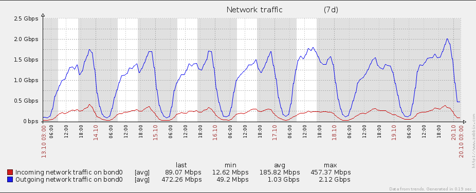
When upgrading the eduroam infrastructure, there was one goal in mind: increase the bandwidth over the previous one. The old infrastructure made use of a Linux box to perform NAT, netflow and firewalling duties. This can all be achieved with dedicated hardware, but the cost was prohibitive and since the previous eduroam solution involved Linux in the centre, the feeling was that replacing like-for-like would yield results faster than would more exotic changes to infrastructure.

This post aims to discuss a little bit about the hardware purchased, and the configuration parameters that were altered in order to have eduroam route traffic above 1Gb/s, which was our primary goal.

Blinging out the server room: Hardware

When upgrading hardware, the first thing you should do is look at where the bottlenecks are on the existing hardware. In our case it was pretty obvious:

  • Network I/O – We were approaching the 1Gb/s limit imposed by the network card on the NAT box (the fact that nothing else in the system set a lower limit is quite impressive and surprising, in my opinion).
  • RAM – The old servers were occasionally hitting swap usage (i.e. RAM was being exhausted). The majority of this is most likely due to the extra services required by OWL but eduroam would have been taking up a non negligible share of memory too.
  • Hard disk – The logging of connection information could not be written to the disk fast enough and we were losing data because of this.

In summary, we needed a faster network card, faster disks and potentially more RAM. While we’re at it, we might as well upgrade the CPU!

Component Old spec New spec
CPU Intel Xeon 2.50GHz Intel Xeon 3.50GHz
RAM 16GB DDR2 667MHz 128GB DDR3 1866MHz
NIC Intel Gigabit Intel X520 10Gb
Disk 32GB 7200 HDD 200GB Intel SLC SSD

Obviously just these four components do not a server make, but in the interests of brevity, I will omit the others. Similarly details outside of the networking stack such as RAID configuration and filesystem are not discussed.

Configuring Linux for peak performance

Linux’s blessing (and its curse) is that it can run on pretty much every architecture and hardware configuration. Its primary goal is to run on the widest range of hardware, from the fastest supercomputer to the netbook (with 512MB RAM) on which I’m writing this blog post. Similarly Debian is not optimized for any particular server hardware nor any particular role, and its packages have default configuration parameters set accordingly. There is some element of introspection at boot time to change kernel parameters to suit the hardware, but the values chosen are always fairly conservative, mainly because the kernel does not know how many different services and daemons you wish to run on the one system.

Because of this, there is great scope for tuning the default parameters to tease out better performance on decent hardware.

Truth be told I suspect this post is the one of the series which most people want to read, but at the same time it is the one I least wanted to write. I was assigned the task of upgrading the NAT boxes so that it removed the bottleneck with ample headroom but, perhaps more crucially, it did so as soon as possible. When you have approximately 2 configuration parameters to tune, the obvious way of deciding the best combination is to test them under load. There were two obstacles in my way. Firstly, the incredibly tight time constraints left little breathing space to try out all configuration combinations I wished. Ideally I would have liked to benchmark all parameters to see how each affected routing. The second (and arguably more important) obstacle was we don’t have any hardware capable of generating 10G worth of traffic on which to create a reliable benchmark.

For problem 2, we tried to use the standby NAT box as both the emitter and collector, but found it incredibly difficult to have Linux push packets out one interface for an IP address that is local to the same system. Said another way, it’s not easy to send data destined for localhost out a physical port. In the end we fudged it by borrowing a spare 10G network card from a friendly ex-colleague and put it into another spare Linux server. With more time, we could have done better, but I’m not ashamed to admit these shortcomings of our testing. At the end of the project, we were fully deployed two weeks late (due to factors completely out of our control), which we were still pleased with.

Aside: This is not a definitive list, please make it one

The following configuration parameters are a subset of what was done on the Linux eduroam servers which in turn is a subset of what can be done on a Linux server to increase NAT and firewall performance. Because of my love of drawing crude diagrams, this is a Venn diagram representation.

A pointless Venn diagram to inject some colour into this blog post

A Venn diagram showing the relationship between the parameters that are available, those modified for our purposes and those discussed in this blog post.

If after reading this post you feel I should have included a particular parameter or trick, please add it as a comment. I’m perfectly happy to admit there may be particular areas I have omitted in this post, and even areas I have neglected to explore entirely with the deployed service. However, based on our very crude benchmarks touched upon above, we’re fairly confident that there is enough headroom to solve the network contention problem at least in the short to medium term.

Let’s begin tweaking!

In the interests of brevity, I will only write configuration changes as input at the command line. Any changes will therefore not persist across reboots. As a general rule, when you see

# sysctl -w kernel.panic=9001

please take the equivalent line in /etc/sysctl.conf (or similar file) to be implied.

kernel.panic = 9001

Large Receive Offloading (LRO) considered harmful

First configuration parameter to tweak is LRO. Without disabling his, NAT performance will be sluggish (to the point of unusable) for even one client connected. Certainly when using the ixgbe drivers required for our X520 NICs we experienced this.

What is LRO?

When a browser is downloading an HTML web page, for example, it doesn’t make sense to receive it as one big packet. For a start you will stop any other program from using the internet while the packet is being received. Instead the data is fragmented when sent and reconstructed upon receipt. The packets are mingled with other traffic destined for your computer (otherwise you wouldn’t be able to load two webpages at once, or even the HTML page plus its accompanying CSS stylesheet.)

Normally the reconstruction is done in software by the Linux kernel, but if the network card is capable of it (and the X520 is), the packets are accumulated in a buffer before being aggregated into one larger packet and passed to the kernel for processing. This is LRO.

If the server were running an NFS server, web server or any other service where the packets are processed locally instead of forwarded, this is a great feature as it relieves the CPU of the burden of merging the packets into a data stream. However, for a router, this is a disaster. Not only are you increasing buffer bloat, but you are merging packets to potentially above the MTU, which will be dropped by the switch at the other end.

Supposedly, if the packets are for fowarding, the NIC will reconstruct the original packets again to below the MTU, a process called General Receive Offload (GRO). This was not our experience and the Cisco switches were logging packets larger than the MTU arriving from the Linux servers. Even if the packets aren’t reconstructed to their original sizes, there is a process called TCP Segmentation Offload (TSO) which should at least ensure a below MTU packet transfer. Perhaps I am missed something, but these features did not work as advertized. It could be related to the bonded interfaces we have defined, but I cannot swear to it.

I must give my thanks again to Robert Bradley who was able to dig out an article on this exact issue. Before that in testing I was seeing successful operation, but slow performance on certain hardware. My trusty EeePC worked fine, but John’s beefier Dell laptop fared less well, with pretty sluggish response times to HTTP requests.

How to disable LRO

The ethtool program is a great way of querying the state of interfaces as well as setting interface parameters. First let’s install it

# apt-get install ethtool

And disable LRO

# for interface in eth{4,5,6,7}; do
>     ethtool -K $interface lro off
> end
#

In fact, there are other offloads, some already mentioned, that the card does that we would like to disable because the server is acting as a router. Server fault has an excellent page on which we based our disabling script.

If you recall in the last blog post I said that eth{4,5,6,7} were defined in /etc/network/interfaces even though they weren’t necessary for link aggregation. This is the reason. I added the script to disable the offloads in /etc/network/if-up.d, but because the interfaces were not defined in the interfaces file, the scripts were not running. Instead I defined the interfaces without any addresses, and now the LRO is disabled as it should be.

# /etc/network/interfaces snippet
auto eth6
iface eth6 inet manual

Disable hyperthreading

Hyperthreading is a buzzword that is thrown around a lot. Essentially it is tricking the operating system into thinking that it has double the number of CPUs that it actually has. Since we weren’t CPU bound before, and since we’ll be setting one network queue per core below, this is a prime candidate for removal.

The process happens in the BIOS and varies from manufacturer to manufacturer. Please consult online documentation if you wish to do this to your server.

Set IRQ affinity of one network queue per core

When the network card receives a packet, it immediately passes it to the CPU for processing (assuming LRO is disabled). When you have multiple cores, things can get interesting. What the Intel X520 card can do is create one queue (on the NIC, containing packets to be handed to the CPU) per core, and pin the queue to interrupt one core. The packets received by the network card are spread across all the queues but packets all share similar properties on a particular queue (the source and destination IP for example). This way, you can make sure that you can keep connections on the same core. This isn’t strictly necessary for us, but it’s useful to know. The important thing is that traffic is spread across all cores.

There is a script that is included as part of the ixgbe source code that is used just for the purpose. This small paragraph does not do such a big topic justice. For further reading please consult the Intel documentation. You will also find other parameters such as Receive Side Scaling that we did not alter but can also be used for fine-tuning the NIC for packet forwarding.

Alter the txqueuelen

This is a hot topic and one which will probably invoke the most discussion. When Linux cannot push the packets to the network card fast enough, it can do one of two things

  1. It can store the packets in a queue (a different queue to the ones on the NICs). The packets are then (usually) sent in a first in first out order.
  2. It can discard the packet.

The txqueuelen is the parameter which controls the size of the queue. Setting the number high (10,000 say) will make for a nice reliable transmission of packets, at the expense of increased buffer bloat (or jitter and latency). This is all well and good if your web page is a little sluggish to load, but time critical services like VOIP will suffer dearly. I also understand that some games require some kind of low latency, although I’m sure eduroam is not used for that.

At the end of the day, I decided on the default length of 1000 packets. Is that the right number? I’m sure in one hundred years’ time computing archaeologists will be able to tell me, but all I can report is that the server has not dropped any packets yet, and I have had no reports of patchy VOIP connections.

Increase the conntrack table size

This configuration tweak is crucial for a network our size. Without altering it our server would not work (certainly not for our peak of 20,000 connected clients).

All metadata associated with a connection is stored in memory. The server needs to do that in order that NAT is consistent for the entire duration of each and every connection, and also that it can report the data transfer size for these connections.

Using their default configuration, the number of connections that our servers can keep track of is 65,536. Right now, as I’m typing this, out of term time, the current number of connections on eduroam is over 91,000. Let’s bump this number:

# sysctl -w net.netfilter.nf_conntrack_max=1048576
net.netfilter.nf_conntrack_max=1048576

At the same time, there is a configuration parameter to set the hash size of the conntrack table. This is set by writing it into a file:

# echo 1048576 > /sys/module/nf_conntrack/parameters/hashsize

The full explanation can be found on this page but basically what is happening is that we are storing a linked list of conntrack entries, but hopefully each list is only one entry long. Since the hashing algorithm is based on the Jenkins hash function, we should ideally choose a power of 2 (220 = 1048576).

This is actually quite a conservative number as we have so much RAM at our disposal, but we haven’t approached anywhere near it since deployment.

Decrease TCP connection timeouts

Sometimes when I suspend my laptop with an active SSH session, I can come back some time later, turn it back on and the SSH session magically springs back to life. That is because the TCP connection was never terminated with a FIN flag. While convenient for me, this can clog up the conntrack table on any intermediate firewall as the connection has to be kept in their conntrack tables. By default the timeout on Linux is 5 days (no, seriously). The eduroam servers have it set to 20 minutes, which is still pretty generous. There is a similar parameter for udp packets, although the mechanism for determining an established connection is different:

# sysctl -w net.ipv4.netfilter.ip_conntrack_tcp_timeout_established=1200
# sysctl -w net.ipv4.netfilter.ip_conntrack_udp_timeout=30

Disable ipv6

Like it or not, IPv6 is not available on eduroam, and anything in the stack to handle IPv6 packets can only slow it down. We have disabled IPv6 entirely on these servers:

# sysctl -w net.ipv6.conf.all.disable_ipv6 = 1
# sysctl -w net.ipv6.conf.default.disable_ipv6 = 1
# sysctl -w net.ipv6.conf.lo.disable_ipv6 = 1

Use the latest kernel

Much work has gone into releases since 3.1 to combat buffer bloat, the main one being BQL which was introduced in 3.6. While older kernels will certainly work, I’m sure that using the latest kernel hasn’t made the service any slower, even though we installed it for reasons other than speed.

Thinking outside the box: ideas we barely considered

As I’m sure I’ve said enough times, getting a faster solution out the door was the top priority with this project. Given more time, and dare I say it a larger budget, our options would have been much greater. Here are some things that we would consider further if the situation allowed.

A dedicated carrier grade NAT box

If the NAT solution posed here worked at line rate (10G) then there wouldn’t be much of a market for dedicated 10G NAT capable routers. The fact they are considerably more expensive and yet people still buy them should probably suggest to you that there is something more to it than buying (admittedly fairly beefy) commodity hardware and configuring it to do the same job. We could also configure a truly high availability system using two routers with something like VSS or MLAG.

The downside would be the lack of flexibility. We have also been bitten in the past when we purchased hardware thinking it had particular features when in fact it didn’t, despite what the company’s own marketing material claimed. Then there is the added complexity of licensing and the recurring costs associated with that.

Load balancing across multiple servers

I touched on this point in the last blog post. If we have ten servers, traffic load balanced evenly across them, they don’t even need to be particularly fast. The problems (or challenges as perhaps they should be called) are the following:

  • Routing – Getting the loads balanced across all the servers would need to be done at the switching end. This would likely be based on a fairly elaborate source based routing scenario.
  • Failover – For full redundancy we would need to have a hot spare for every box, unless you are brave enough to have a standby capable of being the stand-in for any box failing. Wherever you configure the failover, be it on the server itself or the NAT or the switches either side of them, it is going to be complex.
  • Cost – The ten or twenty (cheap) servers are potentially going to be cheaper than a dedicated 10G NAT capable router, but it’s still not going to be cheaper than a server with a 10G NIC (although I admit it’s not the same thing.)

Use BSD

BSD Daemon imageThis may be controversial. I will say now that we here in the Networks team use and love Linux Debian. However, there is a very vocal support for BSD firewalls and routers, and these supporters may have a point. It’s hard to say it tactfully so I’ll just say it bluntly: iptables’s syntax can be a little, ahem, bizarre. The only reason that anyone would say otherwise is because he or she is so used to it that writing new rules is second nature.

Even more controversial would be me talking about speed of BSD’s packet filtering compared with Linux’s, but since that’s the topic of this post, I feel compelled to write at least a few sentences on it. Without running it for ourselves under similar load we are experiencing there is no way to definitively say which is faster for our purposes (the OpenBSD website says as much). The following bullet points can be taken with as much salt as required. The statements are true to the best of my knowledge. Whether the resulting effects will impact performance and to what degree I cannot say.

  • iptables processes all packets; pf by contrast just processes new connections. This is possibly not much of an issue since for most configurations allowing established connections is their first or second rule, but it may make a difference in our scenario.
  • pf has features baked right in that iptables requires modules for. For example pf’s tables look suspiciously like the ipset module.
  • BSD appears to have more thorough queueing documentation (ALTQ) compared with Linux’s (tc). That could lead to a better queuing implementation, although we do not use anything special currently (the servers use the mq qdisc and we have not discovered any reason to change this).
  • Linux stores connection tracking data in a hash of linked lists (see above). OpenBSD uses a red-black tree. Neither has the absolute advantage over the other so it would be a case of try it and see.

Ultimately, using BSD would be a boon because of its easy configuration of its packet filtering. However, In my experience, crafting better firewall rules will result in a bigger speed increase than porting the same rules across to another system. Here in the Networks team we feel that our iptables rules are fairly sane but as discussed in the post on NAT, using the ipset instead of u32 iptables module would be our first course of action should we experience bottlenecks in this area.

Further reading

There are pages that stick out in my mind as being particularly good reads. They may not help you build a faster system, but they are interesting on their respective topics:

  • Linux Journal article on the network stack. This article contains an exquisite exploration of the internal queues in the Linux network stack.
  • Presentation comparing iptables and pf. Reading this will help you understand the differences and similarities between the two systems.
  • OpenDataPlane is an ambitious project to remove needless CPU cycles from a Linux firewall. I haven’t mentioned ideas such as control planes and forwarding (aka data) planes as it is a big subject but in essence, Linux does pretty much all forwarding in the control plane, which is slow. Dedicated routers, and potentially OpenDataPlan can give massive speed boosts to common routing tasks by removing the kernel’s involvement for much of the processing, using the data plane. Commercial products already exist that do this using the Linux kernel.
  • Some people have taken IRQ affinities further than we have, saving a spare core for other activities such as SSH. One such example given is on greenhost’s blog.

In conclusion

In conclusion, there are many things that you can (and you should) do before deploying a production NAT server. I’ve touched on a few here, but again I stress that if you have anything insightful to add, then please add it in the comments.

The next blog post will be on service monitoring and logging.

Posted in eduroam, Firewall, Linux | Tagged , | 3 Comments

Cisco networking & eduroam: Rate Limiting Using Microflow Policing

This is my final post on the interesting technical aspects of the new networking infrastructure that support the eduroam service around the university.

This post covers the finer technical details of how we currently rate limit client devices to 8Mbps download/upload on eduroam – using Microflow Policing on the Cisco 4500-X switches. If readers want to know the reasoning behind why we rate limit at all, then I invite you to read my colleague Rob’s blog post.

Some History

You may recall from my initial blog post that the backend infrastructure that previously supported the eduroam service (and continues to support the OWL service) utilised a dedicated NetEnforcer appliance. This appliance actually did more than simply throttling user connections. In addition, it also performed Deep Packet Inspection (DPI) and applied different policies to certain types of traffic, such as more aggressively throttling P2P traffic for instance.

We had just one of these appliances and this sat inline between the original internal Cisco 3560 switches and the primary Linux firewall host. The appliance utilised an incorporated switch and additional bypass unit. The former providing the required interfaces to connect to the infrastructure, and the latter providing fail-open connectivity in the event of failure.

So you may be asking why we didn’t incorporate the original NetEnforcer hardware into our design? Or why we didn’t acquire upgraded NetEnforcer hardware (or even something from another vendor) to serve our needs moving forward?

Well, the answer to the first question is that the current appliance has reached and gone beyond its end-of-life from the vendor (back in 2013). It has also proved to be prohibitively expensive to purchase and licence during its lifetime, not to mention it’s another ‘bump in the wire’ we would have to manage moving forward.

The answer to the second question is for all the reasons above – plus our default assumption at this point was that a newer 10-gigabit capable appliance from any vendor would only be more expensive, especially if we were to continue to want DPI capabilites. This certainly would not have fitted into our fairly modest budget. Plus with further consideration, we would likely have had to buy two appliances to ensure a truly resilient and reliable service.

In summary, we were searching for an easier way to achieve what we wanted.

So what are we limiting exactly?

At this point, we decided to take a step back and evaluate exactly what bandwidth management we wanted our potential solution to provide. We decided on a goal, which at a high-level, seemed fairly straightforward. That goal was to limit each client device to 8Mbps in both directions. We quickly ruled out the possibility to perform any cleverness with DPI – this would have involved the purchase of additional hardware after all.

To expand on this somewhat and really nail things down, our new solution would have to meet the following requirements:

  • Be capable of identifying, and distinguishing between individual clients connected to the eduroam service;
  • Apply rate-limiting to each client’s overall connection to the network – thus providing a fair and equal service for all that is not based on individual connections or flows, but is based on the sum of each client’s connection;
  • Be implementable using only the hardware/software already procured for the eduroam upgrade;
  • Be implementable without impacting the performance of the infrastructure or the client experience;
  • Be able to scale to the numbers of clients seen today on the service and beyond.

It was these requirements that would lead us to Microflow policing as our preferred method. It might interest readers to note that we also seriously considered using queuing methods on the Linux hosts to achieve this. My colleague Christopher will be writing a blog post on this topic in due course. For now, know that this was a difficult decision that we ultimately made because we had more faith in the scalability of Microflow policing.

QoS Policing vs shaping

Many readers are likely to have heard of the term policing in the context of traffic management. This is used extensively on many service provider networks as an example and the general idea is to limit incoming traffic on an interface, to a certain bandwidth that is less than its capable line rate. Policing can only generally be performed on traffic as it ingresses an interface. It is therefore fundamentally different to another traffic management feature called shaping which is actually concerned with applying queuing methods to rate limit outgoing traffic that egresses interfaces. The terms are often confused and inter-changed so I thought I would attempt to make that distinction as clear as possible before going any further.

The type of policer probably most common (and what we are using in our setup) is often referred to as a one rate, two-colour policer. What this means is that we define a conforming (or allowed) traffic rate in bits per second (bps) called the Committed Information Rate (CIR) and anything over this is considered to have exceeded the CIR. You can then decide on actions for traffic that conforms to, and exceeds your CIR in your policing policy. There are other flavours of policers such as two rate, three colour which allow you to specify a Peak Information Rate (PIR) too and introduces a third violate action. This type of policer could be used to allow traffic to occasionally burst over the CIR within the defined PIR if that were desired, however in our setup it wasn’t really necessary.

Enter Microflow policing

In our case, we didn’t simply need to police all traffic ingressing from the eduroam networks around the university, or vice-versa, from the outside world. We wanted to be far more granular than that as per the requirements above. To enable us to do this, another feature was needed in conjunction to a standard QoS policer. This feature, called Microflow policing, makes use of Flexible Netflow on the Cisco 4500-X switches in conjunction with some configured class-maps and ACLs, to create a granular policy that applies to specific traffic as it enters the eduroam infrastructure from the university backbone and vice-versa, from the outside world (via our firewalls).

Flexible Netflow is a relatively new feature in Cisco’s portfolio that allows you to specify custom records that define exactly which fields within packets you’re interested in interrogating – which fits our purposes very nicely indeed!

Defining how we Identify & distinguish between eduroam clients

To fulfil our requirements above, we had to identify and distinguish our clients on the eduroam service. To do this required the following configuration:

flow record IPV4_SOURCES
 match ipv4 source address

flow record IPV4_DESTINATIONS
 match ipv4 destination address

ip access-list extended EDUROAM_DESTINATIONS
 permit ip any 10.16.0.0 0.15.255.255

ip access-list extended EDUROAM_SOURCES
 permit ip 10.16.0.0 0.15.255.255 any

OK some explanation will likely aid understanding here.

Firstly, the ‘flow record’ commands tell Flexible Netflow to set up two custom records – the ‘IPV4_SOURCES’ one as the name suggests, is set up to read the source address field in the IPv4 packet header and the ‘IPV4_DESTINATIONS’ one is conversely set up to read the destination address field in the IPv4 header.

Next, two extended ACLs are set up to specify the actual IPv4 addresses we’re looking for – traffic traversing the eduroam service! The ‘EDUROAM_SOURCES’ one specifies traffic sourced from within the eduroam client address range 10.16.0.0/12 destined for any address. The ‘EDUROAM_DESTINATIONS’ ACL specifies the exact opposite – specifically, traffic sourced from any address destined for clients within 10.16.0.0/12.

The eagle-eyed amongst you will have realised that I’ve specified the internal eduroam client address range here and not the public range. This is important going forward for two reasons:

  • We use NAT overload to translate the internal RFC 1918 space 10.16.0.0/12 into a much smaller /26 of publicly-routable space (IPv4 address space on the Internet is at a premium after all). Therefore it would be impossible to distinguish individual clients using the public range as one address within this range is likely to actually represent numerous clients. Therefore we have to apply our policies before applying NAT translation;
  • We are now limited (remembering that policing only works in the ingress direction) on which interfaces we can apply our Microflow policing policy to.

Classifying the traffic we’re interested in

So now we’ve specified our parameters for identifying and distinguishing our clients, it’s time to set up some class-maps to classify the traffic we want to manipulate. This is done in the generally accepted, standard Cisco class-based QoS manner. Like this:

class-map match-all MATCH-EDUROAM-DESTINATIONS
 match access-group name EDUROAM_DESTINATIONS
 match flow record IPV4_DESTINATIONS

class-map match-all MATCH-EDUROAM-SOURCES
 match access-group name EDUROAM_SOURCES
 match flow record IPV4_SOURCES

Note that I’ve given the class maps meaningful names that tie in with those that I gave to the ACLs defined above. Also note that I have used the match-all behaviour in the class-maps. So for traffic to match the policy, it has to match both the extended ACL and the flow record statement. In fact, traffic will always match the flow records, as all IPv4 packets have source and destination address headers! This is exactly why we need the ACLs too.

Defining our QoS policy

Now for the fun part! Let’s set up our policy-maps containing the policer statements. There’s nothing particularly fancy going on in this QoS policy configuration – remember the cleverness is really under the hood of our class-maps referencing our custom flow records and ACLs:

policy-map POLICE-EDUROAM-UPLOAD
 class MATCH-EDUROAM-SOURCES
 police cir 8000000
 conform-action transmit
 exceed-action drop

 policy-map POLICE-EDUROAM-DOWNLOAD
 class MATCH-EDUROAM-DESTINATIONS
 police cir 8000000
 conform-action transmit
 exceed-action drop

The policy maps are named differently – but are still meaningful to us. One policy is designed to affect download speeds, so it’s called ‘POLICE-EDUROAM-DOWNLOAD’ and the other is designed to affect upload speeds so is called ‘POLICE-EDUROAM-UPLOAD’.

Tying it all together

So let’s quickly tie this all together. Firstly, pay particular attention to which class-maps I’ve referenced in each policy map. The logic works like this:

  • The ‘POLICE-EDUROAM-UPLOAD’ policy map references the ‘MATCH-EDUROAM-SOURCES’ class-map, which in turn references the ‘EDUROAM-SOURCES’ ACL and ‘IPV4_SOURCES’ flow record, which in turn matches traffic sourced from clients within 10.16.0.0/12 – our eduroam clients;
  • The ‘POLICE-EDUROAM-DOWNLOAD’ policy map references the ‘MATCH-EDUROAM-DESTINATIONS’ class-map, which in turn references the ‘EDUROAM-DESTINATIONS’ ACL and ‘IPV4_DESTINATIONS’ flow record, which in turn matches traffic destined to clients within 10.16.0.0/12 – again, our eduroam clients.

Also note that the CIR has been specified as 8000000bps. The keen mathematicians amongst you will note that this is not actually 8Mbps, but it’s very close. I could have been even more specific and specified 7629395bps but I figured I would round the figures up to make our lives here in Networks a little easier! Also note that I have specified the conform and exceed actions to be transmit and drop respectively. Note that for this to work properly, the conform action must transmit the traffic and the exceed action must be defined or the policy simply won’t do anything useful. It is possible to configure the exceed action to re-mark packets to a lower Differentiated services code point (DSCP) value rather than to drop them if this better matched your own existing QoS policies and you were that way inclined. However, the drop action suits our requirements here.

Applying the policies to the interfaces

This all looks good, but we’re not done yet. The final step in the process was to apply the QoS policy-maps to the correct interfaces:

interface Port-channel10
 service-policy input POLICE-EDUROAM-DOWNLOAD

interface Port-channel11
 service-policy input POLICE-EDUROAM-DOWNLOAD
end
interface Port-channel50
 service-policy input POLICE-EDUROAM-UPLOAD

interface Port-channel51
 service-policy input POLICE-EDUROAM-UPLOAD

So that’s four interfaces in our topology. The first two are the portchannels connecting to the inside interfaces of our Linux firewalls and the others are the portchannels connecting to the university backbone routers. To aid in understanding, I’ve also depicted this on the diagram below:

Eduroam-backend-refresh-Microflow-policing-placement-1.0

Verification

To see this in action, and prove it works, you can always use the speedtest.net method which in fact I did during my initial testing, as I knew that this method would be the yardstick many of my colleagues around he university would be using to test their download and upload speeds when connected to the service.

I won’t bore you with screenshots from speedtest.net, I’m more interested in showing you the output from the 4500-X switches to see what’s actually happening. Here’s some show output from the production lin-router switches as of today:

lin-router#show policy-map interface po10
 Port-channel10
Service-policy input: POLICE-EDUROAM-DOWNLOAD
Class-map: MATCH-EDUROAM-DESTINATIONS (match-all)
 361805297845 packets
 Match: access-group name EDUROAM_DESTINATIONS
 Match: flow record IPV4_DESTINATIONS
 police:
 cir 8000000 bps, bc 250000 bytes
 conformed 408690519012173 bytes; actions:
 transmit
 exceeded 26635280726176 bytes; actions:
 drop
 conformed 303156000 bps, exceeded 19320000 bps
Class-map: class-default (match-any)
 1998983 packets
 Match: any

lin-router#show policy-map interface po50
 Port-channel50
Service-policy input: POLICE-EDUROAM-UPLOAD
Class-map: MATCH-EDUROAM-SOURCES (match-all)
 253107616302 packets
 Match: access-group name EDUROAM_SOURCES
 Match: flow record IPV4_SOURCES
 police:
 cir 8000000 bps, bc 250000 bytes
 conformed 73378531150889 bytes; actions:
 transmit
 exceeded 613359041557 bytes; actions:
 drop
 conformed 75872000 bps, exceeded 471000 bps
Class-map: class-default (match-any)
 332605099 packets
 Match: any

This output serves to provide us with information that tells us:

  • The QoS policy applied;
  • What packets it has been configured to match;
  • What the policy will do to the packets;
  • What packets conformed to the CIR and what action was taken;
  • What packets exceeded the CIR and what action was taken.

The output above of course only shows the primary path through the infrastructure. The non-zero values here indicate that our policies are acting on our traffic to and from eduroam clients. Success!

Final thoughts & points to note

So this does work very nicely in our scenario. However there were some things to take into account when contemplating using the Microflow policing feature and I suggest anyone also thinking about it consider the following points:

  • Plan your policies carefully before even touching a terminal – make sure you have a good handle on what flow records you’ll need to create and any associated ACLs or other configuration you’ll need;
  • Plan the placement of policies carefully – making sure you use the correct interfaces and remember that policing is an ingress action!
  • Make sure you select a Cisco platform with a large enough TCAM that holds enough Netflow entries – if you’re using switches in a VSS pair and MECs that connect across them like we did, then provided you’re load-sharing traffic between the physical switches relatively evenly (check which hashing algorithm your chosen channeling protocol is using for example), you could safely combine the Netflow TCAM capacity sizes of both switches and work with that figure as each physical switch’s own Netflow engine processes traffic independently;
  • Watch out for any existing Netflow configuration on interfaces – you cannot apply a ‘service-policy’ configuration to an interface already configured with ‘ip flow monitor’ for example.

Finally, bear in mind that the configuration listed here is what was applied to the 4500-X platform. Readers may find the configurations here are also useful for other platforms running IOS-XE, but you may also find some differences too!

Some platforms running IOS that support Flexible Netflow may also support the Microflow policing feature, though the configuration syntax is likely to be vastly different. Therefore I would always recommend you check out the Feature Navigator and other documentation available at cisco.com (will require a CCO login) for more information.

Many thanks for reading!

Posted in Cisco Networks, eduroam | 1 Comment

Linux and eduroam: link aggregation with LACP bonding

A photo of two bonded linksIn previous posts, I discussed the roles of routing and NATing in the new eduroam infrastructure . In one sense, that is all you need to create a Linux NAT firewall. However, the setup is not very resilient. The resulting service would be littered with single points of failure (SPoF), including:

  • The server – Reboots would take the service down, for example when installing a new kernel.
  • Ethernet cables – With one cable leading to “inside” the eduroam network and and one cable leading to “the outside world”, it would only take either cable to develop a fault to result in a complete service outage.

Solving the first SPoF is easy (at least for me)! I can just install two Linux boxes, identical to each other, and leave John to figure out how to route the traffic to each. We currently have an active-standby set up where all traffic flows through one box until the event that the primary is unavailable. No state is shared between these boxes currently, which means that a backup server promoted to active duty will result in lost connection data and DHCP leases. Because of this we will only do kernel reboots during our designated Tuesday morning at-risk period unless there is good reason to do otherwise. State sharing of connection data and DHCP leases is possible but we would have to weigh up the advantages against the added complexity of configuration and the added headache of maintaining lock step between the two servers.

As you may have guessed from its title, this blog post is going to discuss bonding, which (amongst other things) solves the problem of having any single cable fail.

Automatic fail over of multiple links

When you supplement one ethernet cable with another on Linux, you have a number of configuration choices for automatic failover, so that when one cable goes down all traffic goes through the remaining cable. When taking into account that the other end is a Cisco switch, the choices are narrowed slightly. Here are the two front runners:

Equal-cost multi-path routing (ECMP, aka 802.1Qbp)

Multipath routing is where multiple paths exist between two networks. If one path goes down, the remaining ones are used instead.

Each route is assigned a cost. The route with the lowest overall cost is chosen. When a link goes down, a new path is calculated based on the costs of the remaining routes. This can take a noticeable amount of time. However, with multiple routes having the same cost, the failover can be near instantaneous. The multiple routes can be used to increase bandwidth, but our main goal is resiliency.

As a point of interest, our previous eduroam (and current OWL) infrastructure uses multipath (not equal-cost) to fail over between the active and standby NAT boxes. On either side of these two boxes sits a switch and across these two switches is defined two routes, one through the active NAT server, the other through the standby. The standby has a higher cost by virtue of an inflated hop count so all traffic flows through the active. A protocol called RIPv2 is used to calculate route costs and when a link goes down, the switches re-evaluate the costs of routing traffic and decide to send traffic through the standby. This process takes approximately 5 seconds.

OWL routing has RIPv2 going through two NAT servers, each route having a different cost. When the primary link goes down, the routes are recalculated and all traffic subsequently flows through the standby path, which has an inflated hop count to create a higher routing cost.

OWL routing has RIPv2 going through two NAT servers, each route having a different cost. When the primary link goes down, the routes are recalculated and all traffic subsequently flows through the standby path, which has an inflated hop count to create a higher routing cost.

The new eduroam switches use object tracking to manage fail over of the individual servers. This is independent of link aggregation explained below.

Link Aggregation Control Protocol (LACP, aka 802.3ad, aka 802.1ax, aka Cisco Etherchannel, aka NIC teaming)

This is the creation of an aggregation group so that the OS would present the two cables as one logical interface (e.g. bond0). This makes configuration of the NAT service much simpler as there is only one logical interface to worry about when configuring routes and firewall rules.

ECMP has its advantages (for one, the two links can be different speeds and can span across multiple Linux firewalls [see MLAG below]), but LACP is the aggregation method of choice for many people and we were happy to go with convention on this one.

The name’s bond, LACP bond

LACP links are aggregated into one logical link by sending LACPDU packets (or, more accurately, LACPDU frames if you have read the previous blog post) down all the physical links you wish to aggregate. If an LACPDU reply is subsequently received from the device at the other end, then the link is active and added to the aggregation group. At the same time, each interface is monitored to make sure that it is up. This happens much more frequently and is used to check the status of the cables between the two devices. After all, you are more likely to suffer a cut cable scenario than a misconfiguration once everything is set up and deployed.

How traffic is split amongst the different physical cables will be discussed later but for now it suffices to say that all active cables can be used to transmit traffic so if you have two 1Gb links, the available bandwidth is potentially 2Gb. While some people aggregate links for increased bandwidth, we are solely using it for improved resiliency. Any increased throughput is a bonus.

When receiving traffic through bonded interfaces, you do not necessarily know through which physical interface the sending device sent them; the decision rests solely on the sending device. However, there are some assumptions that are fairly safe, like all traffic for a single connection is sent via the same physical interface (subject to the link not going down mid connection, obviously.)

How can you use it? A simplified picture

Two devices communicating using a bonded connection of two cables will use both those cables to transmit data, failing over gracefully should any one cable fail. In fact you are not limited to two cables. The LACP specification says that up to eight cables can be used (link-id, which is unique for each physical interface can be an integer between 1 and 8.) In reality four may be a lower limit imposed by your hardware.

A schematic diagram of how the switches either side of the NAT server are connected using bonding is shown below.

A diagram of LACP bonding. There are two lines for every connection, with each pair with a circle enveloping them

A simplistic view of how link aggregation is represented for eduroam using standard drawing conventions

Here we see two links either side of the NAT server, with circles around them. This is the convention for drawing a link aggregation.

How do we use it? The whole picture

In reality the diagram above is incomplete. The new eduroam service is designed to be a completely redundant system. Every connection has two links aggregated and every device is replicated so that no one cable nor device can bring down the service. In fact, with every link aggregated and there being a backup server, a minimum of four cables would need to fail for the service to go down, up to a possible six.

Below is a diagram of all the link aggregations in action.

A diagram to show the complex provisioning of link aggregation for Oxford University's eduroam deployment

The full picture of where we use link aggregation for eduroam.

This diagram is a work of art (putting to shame my felt-tip pen efforts) created by John and described in his earlier blog post. I would recommend reading that blog post if you wish to understand the topology of the new eduroam infrastructure. However, this blog series takes a look at the narrow purview of what the Linux servers should be doing, and so no real understanding of the eduroam topology is required to follow this.

Installing and setting up LACP bonding on Debian Linux

I should point out that nothing I am saying here cannot be gleaned from the Linux kernel’s official documentation on the subject. That document is well written and very thorough. If I say anything that contradicts that, then most likely it is me in error. In a similar vein, you can find a great number of blog posts on link aggregation that contradict the official documentation and each other.

As an example, you will encounter conflicting advice about the use of ifenslave to configure bonding. For example, some posts will say that it is the correct way of doing things, others will say that its use is deprecated and that you should use iproute2 and sysfs.

Which is correct? Well, for Debian (which we use) it’s a mixture of both. As I understand it, there was a program ifenslave.c that used to ship with Linux kernels which handled bonding. This is now deprecated. However, Debian has a package called ifenslave-2.6 which is a collection of shell scripts which are run to help create a bonded interface from the configuration files you supply. In theory you can dispense with these scripts and configure the interface yourself using sysfs, but I wouldn’t recommend it. These scripts are placed in the directories under /etc/network and are run for every interface up/down event.

So, with that in mind, let’s install ifenslave-2.6:

apt-get update && apt-get install ifenslave-2.6

Now we can define a bonded interface (let’s call it bond0) in the /etc/network/interfaces file. This file does not need to have the eth5, eth7 devices defined anywhere else in the interfaces file (we do define them, for reasons to be explained in, you guessed it, a later blog post.)

auto bond0
iface bond0 inet static
        bond-slaves eth7 eth5
        address  192.168.34.97
        netmask  255.255.255.252
        bond-mode 802.3ad
        bond-miimon 100
        bond-downdelay 200
        bond-updelay 200
        bond-lacp-rate 1
        bond-xmit-hash-policy layer2+3
        txqueuelen 10000
        up   /etc/network/eduroam-interface-scripts/bond0/if-up
        down /etc/network/eduroam-interface-scripts/bond0/if-down

Let’s get rid of the cruft so that just the relevant stanzas remain (the up/down scripts are for defining routes and starting and stopping the DHCP server.)

iface bond0 inet static
        bond-slaves eth7 eth5
        bond-mode 802.3ad
        bond-miimon 100
        bond-downdelay 200
        bond-updelay 200
        bond-lacp-rate 1
        bond-xmit-hash-policy layer2+3

All these lines are very well described in the official documentation so I will not explain anything here in any depth, but to save you the effort of clicking that link, here is a brief summary:

  • LACP bonding (bond-mode).
  • Physical links eth5 and eth7 (bond-slaves).
  • Monitoring on each physical link every 100 milliseconds (bond-miimon), with a disable, enable delay of 200 milliseconds (bond-downdelay, bond-updelay) should the link change state.
  • Aggregation link checking every second (bond-lacp-rate). The default is 30 seconds which probably would suffice, but it means misconfigurations are detected faster.

The one option I have left out is the bond-xmit-hash-policy which probably needs a fuller explanation.

bond-xmit-hash-policy

I said earlier that I would explain how traffic is split across the physical links. This configuration option is it. In essence the Linux kernel is using a packet’s properties to assign a number to it (link-id), which is then mapped to a physical cable in the bond. Ideally you would want each connection to go through one cable and not be split.

The default configuration option is “layer2” which uses the source and destination MAC address to determine the link. Bonded interfaces share a MAC address across their physical interfaces on Linux, so when the two ends are configured as a linknet comprising just two hosts, there are only two MAC addresses in use, those of the source and destination. In other words, all traffic will be sent down one physical link!

Now, this would be fine. Our bonding is used for resilience, not for increased bandwidth and since the NICs are 10Gb capable Intel X520s, there should be enough bandwidth to spare (we currently peak at around 1.7Gb/s in term time.)

However, we would prefer to use both links evenly if possible for reasons of load balancing the 4500-X switches at the other end of the cables. We use microflow policing on the Cisco boxes and as I understand it, these work better with an even distribution of traffic. For that reason, we specify a hash-policy of layer2+3 which includes the source and destination IP addresses to calculate the link-id. The official documentation has an explanation of how this link-id is calculated for each packet.

Monitoring LACP bonding on Debian Linux

True to Unix’s philosophy of “everything is a file”, you can query the state of your bonded interface by looking at the contents of the relevant file in /proc/net/bonding:

$ cat /proc/net/bonding/bond0
Ethernet Channel Bonding Driver: v3.7.1 (April 27, 2011)

Bonding Mode: IEEE 802.3ad Dynamic link aggregation
Transmit Hash Policy: layer2+3 (2)
MII Status: up
MII Polling Interval (ms): 100
Up Delay (ms): 200
Down Delay (ms): 200

802.3ad info
LACP rate: fast
Min links: 0
Aggregator selection policy (ad_select): stable
Active Aggregator Info:
        Aggregator ID: 1
        Number of ports: 2
        Actor Key: 33
        Partner Key: 11
        Partner Mac Address: 02:00:00:00:00:63

Slave Interface: eth7
MII Status: up
Speed: 10000 Mbps
Duplex: full
Link Failure Count: 2
Permanent HW addr: a0:36:9f:37:44:da
Aggregator ID: 1
Slave queue ID: 0

Slave Interface: eth5
MII Status: up
Speed: 10000 Mbps
Duplex: full
Link Failure Count: 2
Permanent HW addr: a0:36:9f:37:44:ca
Aggregator ID: 1
Slave queue ID: 0

Here we can see basically the same configuration we put into /etc/network/interfaces along with some useful runtime information. A particularly useful line is the Link Failure Count, which shows that both physical links have failed twice since the last reboot. As long as these failures did not occur simultaneously across the two physical links, the service should have remained on the primary server (which it did.)

Notice how there isn’t an IP address in sight. This is because LACP is a layer 2 aggregation so it does not need to know about any IP address to function. The IP addresses we configured in /etc/network/interfaces are those built on top of LACP and are not part of LACP’s function.

What they don’t tell you in the instructions

So far so good. If you’re using this blog post as a step by step guide, you should successfully have bonding so that any link in an aggregation can go down and you wouldn’t even notice (unless your monitoring system is configured to notify you of physical link failure.)

However, there are some things that tripped me up. Hopefully by explaining them here I will save a little headache for anyone who wishes to tread a similar path to mine.

Problem 1: Packet forwarding over bonded links

By default, Linux has packet forwarding turned off. This is a sensible default, one we’d like to keep for all interfaces (including management interface eth0), except for the interfaces we require to forward: bond0 and bond1. You can configure this, as we’ve done using sysctl.conf

net.ipv4.conf.default.forwarding=0
net.ipv4.conf.eth0.forwarding=0
net.ipv4.conf.bond0.forwarding=1
net.ipv4.conf.bond1.forwarding=1

Now looking at this, you’d think this would work, and that eth0 wouldn’t forward packets but bond0 and bond1 will.

Wrong! What actually happens is that neither bond0 nor bond1 will forward packets after a reboot. What’s going on? It’s a classic dependency problem, and one that has been in Debian for many years. The program procps, which sets up the kernel parameters at boot, runs before the bonding drivers have come up. The Debian wiki has solutions, of which the one we picked is to run “service procps reload” again in /etc/rc.local. Yes, you do still get error messages at boot and there is a certain whiff of a hack about this, but it works and I’m not going to argue with a solution that works and is efficient to implement, no matter how inelegant.

Problem 2: Traffic shaping on bonded links

This really isn’t a problem I was able to solve. In the testing phases of the new eduroam, we looked at traffic shaping using the Linux boxes and the tc command. We could get this to reliably shape traffic for physical interfaces, but applying the same queueing methods on bond0 proved far too unreliable. There are reports [1][2] that echo my experiences, but even running the latest kernel (3.14 at the time of deployment) did not fix this, nor did any solutions that I found on the web. In the end we abandoned the idea of traffic shaping on the Linux boxes and instead used microflow policing on the Cisco 4500-X switches, which as it happens works very well.

I hope to write at least a summary of traffic shaping on Linux as it’s considered a bit of a dark art and although I didn’t actually get anywhere with it, hopefully I can impart a few things I learnt.

Problem 3: Mysterious dropped packets

You may remember me mentioning in the last blog post that we backported the Jessie kernel into these hosts. The reason wasn’t a critical failure of the Wheezy default kernel, but it irked me enough to want to remedy it.

Before kernel release 3.4, there was a bug where LACPDU packets were received and processed, but then discarded as an unknown packet by the kernel, in the process incrementing the RX dropped packets counter. This counter is an indicator that something is wrong, so seeing this number increment at a rate of several a second is quite alarming. The bug was fixed in 3.4 (main patch can be found at commit 13a8e0.) Unfortunately Debian Wheezy uses kernel 3.2 by default. The solution was to install a backported kernel. We have not experienced any increase in server reboots because of this, although the possibility of course is there as Jessie is a constantly moving target.

Running 3.14 for the past 35 days, we have forwarded around 200000000000 packets, and dropped 0! For those interested, 2× 10¹¹ packets is, in this instance, 120TB of data.

What I looked into but didn’t implement

As is becoming traditional with this blog series, here are a few things that I looked into, but for some reason didn’t implement (mostly time constraints). Usual caveats apply.

Clustered firewall

At the moment we have a redundant setup. If the primary NAT server falls over, or goes offline, the secondary will receive traffic. The failover is 2 seconds and we hope that is fast enough for an event that doesn’t occur too often (the old servers have an uptime of 400 days and counting.)

When the failover happens, the secondary starts with a completely blank connection tracking table, which is filled as new connections are established. This means that already existing connections are terminated by the NAT firewall and have to be re-established.

However, it is possible to share connection tracking data between these two servers. This means that should the primary go down, the secondary should be able to NAT already established connections, and all people will notice is a two second gap when data is streamed.

This functionality is provided by conntrackd, which is part of the netfilter suite of tools. If we were to use it, we would even be able to provide active-active NAT thereby spreading the bandwidth across both servers. It’s something we can consider in the future, but at the moment, it’s overkill for our needs.

Multi-Chassis link aggregation (MLAG)

When I said above that the LACP we have implemented was to protect us from a faulty cable, I was in fact omitting a rather big fact. The cables from the Linux server actually go to two separate Cisco 4500-X switches so in other words, not only is it guarding against a failed cable, but also a failed switch. Eagled eyed readers may already have spotted this in John’s diagram above.

Now normally this isn’t possible because LACP requires all physical interfaces to be on the same box, but this is a special case. The two boxes are set up as a VSS pair which means that the two physical boxes are presented as one logical switch. When one physical switch fails, the logical switch will lose half its ports, but otherwise will carry on as if nothing has happened.

Now, with this conntrackd daemon I mentioned above, is it possible to achieve a similar effect with two Linux servers, where a bond0’s slave interfaces are shared across multiple physical servers? Well, in a word, no. MLAG is a relatively new technology and as such has been implemented differently by different vendors using proprietary techniques. We use Cisco’s VSS, but even Cisco themselves they have multiple technologies to achieve the same effect (vPC). Until there is a standard on which Linux can base its implementation, it’s unlikely one will exist.

In Linux’s defence, there are ways around this. You could set up your cluster with ECMP via the switches either side of them, and any link that fails gets its traffic rerouted through the remaining links. The conntrackd would mean that the connection would stay up. However this is speculation as I haven’t tried this.

Coming up next

That concludes this post on bonding. Coming up next is a post on buying hardware and tuning parameters to allow for peak performance.

Posted in eduroam, Linux | Tagged , , , | 8 Comments

Configuring Cisco Ethernet management interfaces

Following on from recent posts where I have covered our use of the Cisco Catalyst 4500-X platform for the eduroam networking infrastructure upgrade project, I thought it would be good to cover the Ethernet management interface in more detail. Why, I hear you ask? Well, whilst the topic in itself probably seems very trivial (and a bit dull frankly), configuring this and getting it to actually work proved trickier than I initially expected!

Having spent some time researching the topic online after hitting a few snags, I wasn’t able to find one single resource that answered all my questions.

Therefore my hope is that this post may prove a useful time-saver to those who find themselves with a Cisco switch or router with an ethernet management interface they wish to use for management and monitoring systems.

Why should you use the management interface at all?

This is a valid question. In some scenarios you may decide you don’t wish to. Certainly with the majority of our Cisco switching estate, we choose not to either. In cases where we *must* have Out-Of-Band (OOB) access to a device in the event of a major outage (thankfully we don’t see many of those), we often instead favour the use of the console port connected with terminal servers which we can connect to over an alternative IP network. For other cases, we often use one of the standard base T ports VLAN’d off onto a separate Lights Out Management (LOM) network.

However using this dedicated management interface can be of benefit for many reasons depending on the scenario you’re working with. Here are few of the main ones that influenced our decision in the case of the 4500-X platform:

  • It isolates management traffic away from the global routing table in a dedicated VRF;
  • It avoids having to use ‘front-facing’ interfaces;
  • It avoids the expense of having to procure extra base T transceivers if you’re working with an all SFP/SFP+ platform.

I’m sure there are other benefits too of course, though being that the 4500-X is an all SFP platform with no other built-in base T ports, this seemed like a very sensible way to go.

Overview of management configuration – things to note

So, when I initially found myself sat at a terminal attempting an initial configuration of one of these switches, I quickly realised that our standard configuration template wasn’t going to cut the mustard. I found some caveats with how you might normally expect to configure features, even the basic things.

Here’s a summary of what I found. I’ll expand on these later on in this post:

  • The management port out-of-the box is assigned to a management VRF (called ‘mgmtVrf’ or some variation depending on the platform and software version you’re working with) and cannot be re-assigned to either another VRF, or the global routing table (so you can’t cheat);
  • We restrict VTY lines on our devices using an ACL to limit access to defined management IP hosts/networks. I found that without an additional parameter in the access-class configuration statement I got ‘connection refused’ errors when attempting to connect to the VTY line;
  • Rather counter-intuitively, using the ‘vrf <vrfname>’ variant of the ip domain-name command needed for Secure Shell (SSH) configuration did not work when generating crypto keys;
  • Authentication Authorisation & Accounting (AAA) configurations using the ‘default’ server group would not work;
  • A custom AAA server group had to be defined for TACACS+/RADIUS servers. Within this I had to use some specific commands to get this to work including specifying the source interface for associated requests;
  • Some common global configuration mode commands could be used as normal, but others required the mgmtVrf VRF to be configured as an additional parameter;

See? I told you it was tricky!

SSH/VTY configuration

As described earlier, the sensible thing to do is to restrict access to your devices to only use SSH and only be allowed to do so from certain authorised hosts/networks.

In light of this, here’s what our basic configuration looks like (I’ve changed some IPs to dummy ones for security reasons):

aaa new-model

username networks secret <password>

ip domain-name lom.oucs.ox.ac.uk

ip access-list standard SSH-ACCESS
 permit 192.168.3.222
 permit 192.168.1.67
 permit 192.168.102.0 0.0.0.31
 permit 192.168.21.0 0.0.0.255
 permit 192.168.22.0 0.0.0.255
 permit 172.16.0.0 0.0.15.255
 permit 192.168.2.0 0.0.0.255

ip ssh time-out 60
ip ssh source-interface <source-interface>
ip ssh version 2

line vty 0 4
 access-class SSH-ACCESS in
 exec-timeout 5 0
 logging synchronous
 transport input ssh

line vty 5 15
 exec-timeout 0 0
 logging synchronous
 transport input none

Then of course, we would generate the RSA key:

crypto key generate rsa general-keys modulus 2048

OK, this part of the configuration has probably changed the least in light of using the management port.

I’d like to highlight that using the following command as a substitute for the one above did not work:

ip domain-name vrf mgmtVrf lom.oucs.ox.ac.uk

Great! This is really counter-intuitive isn’t it?  Using the VRF-specific variant of the command instead of the standard command will mean you won’t be able to generate the RSA key. However, you do need this command in addition to allow DNS lookups assuming you want to do this via the management interface too in conjunction with VRF-specific name server commands.

The only remaining changes necessary to allow this part of the configuration to work was the addition of two commands within the line vty configuration:

line vty 0 4
 access-class SSH-ACCESS in vrf-also
 exec-timeout 5 0
 logging synchronous
 login authentication TAC_PLUS
 transport input ssh

line vty 5 16
 exec-timeout 0 0
 logging synchronous
 transport input none

With these changes in place, you should be able to generate the RSA key as normal and find that SSH access via the VTYs works as expected. These are only very subtle differences granted, but I suspect you may find yourself scratching your head for a while without them – I certainly did!

The configuration of the specific custom AAA server group (named TAC_PLUS in my examples) is detailed in the next section. If in your own scenario you simply rely on the local database for authentication, then you shouldn’t need the ‘login authentication’ command.

AAA configuration

You can probably ignore this section if you aren’t using AAA – ie. if you don’t use a TACACS+ or RADIUS server to manage access to your network devices. In all likelihood, I would imagine you would be using one or the other in most cases.

Our default AAA configuration is pretty standard really. In the case of normal operation, any users wishing to log into a network switch for example, are required to authenticate via our team-internal TACACS+ service, which in-turn decides what level of access a user is allowed (full or read-only) and what commands they are allowed to enter. This service also keeps accounting records – i.e. what a user did whilst they were logged in to a switch.

In the rare case where the TACACS+ server may be unavailable, users can authenticate via the local user database on the switch. This should only ever be the case if the TACACS+ method is unavailable.

These rules should also be applied regardless of where a user logs in from – i.e. whether they log in remotely over a VTY line or if they are attached directly to the console port of the switch.

So with all this in mind, our normal AAA configuration template looks like this:

aaa authentication login default group tacacs+ local
aaa authentication enable default enable group tacacs+
aaa authorization console
aaa authorization exec default group tacacs+ local 
if-authenticated
aaa authorization commands 15 default group tacacs+ local 
if-authenticated
aaa accounting commands 1 default stop-only group tacacs+
aaa accounting commands 15 default stop-only group tacacs+

tacacs-server host <tacacs-server-IP> key <key-string>
tacacs-server directed-request

ip tacacs source-interface <source-interface>

This configuration didn’t work at all when using the management interface. Instead, you have to first define your own server group like this:

aaa group server tacacs+ TAC_PLUS
 server-private <tacacs-server-IP> key <key-string>
 ip vrf forwarding mgmtVrf
 ip tacacs source-interface <management-interface>

In fairness, Cisco have been warning us for quite some time that they would be deprecating the old ‘tacacs-server’ and ‘radius-server’ commands. Old habits often die hard though!

Also note the use of the ‘server-private’ command and the definition of the mgmtVrf VRF within the group. Both are important!

In light of our new custom AAA server group configuration, the AAA method commands also have to be amended to match. These now should look something like this (exact commands may vary depending on your own AAA policies used locally of course):

aaa authentication login default group TAC_PLUS local
aaa authentication enable default group TAC_PLUS enable
aaa authorization console
aaa authorization exec default group TAC_PLUS local 
if-authenticated
aaa authorization commands 15 default group TAC_PLUS local 
if-authenticated
aaa accounting commands 1 default stop-only group TAC_PLUS
aaa accounting commands 15 default stop-only group TAC_PLUS

Other global configuration mode commands

There are of course other management services to consider, assuming of course, you want all management-related traffic to utilise the management port.

Commands for these other services are entered in global configuration mode. Using the dedicated management port, some of these commands have to be amended to include additional parameters whereas others do not. I would suggest that using the context-help (our helpful friend the ‘?’) in IOS/IOS-XE will help here in addition to the configuration guide for your platform.

Here’s how I configured the 4500-X platform to send queries to our DNS servers, send logs to our syslog server, participate in SNMP and synchronise its clock to our NTP servers via the management port. I’ve highlighted in bold the commands that have to be amended:

ip domain-name vrf mgmtVrf lom.oucs.ox.ac.uk
ip name-server vrf mgmtVrf <dns-server-1-IP>
ip name-server vrf mgmtVrf <dns-server-2-IP>
ip name-server vrf mgmtVrf <dns-server-3-IP>

logging trap debugging
logging facility local6
logging host <syslog-server-IP> vrf mgmtVrf

snmp-server community <community-string> RO 
<restricted-ACL-name/number>
snmp-server trap-source <management-interface>
snmp-server source-interface informs <management-interface>
snmp-server contact Networks
snmp-server host <snmp-poller-IP> vrf mgmtVrf 
<community-string/username>  tty vtp config vlan-membership snmp
snmp-server host <snmp-poller-IP> vrf mgmtVrf 
<community-string/username  tty vtp config vlan-membership snmp

ntp source <management-interface>
ntp server vrf mgmtVrf <ntp-server-1-IP>
ntp server vrf mgmtVrf <ntp-server-2-IP>
ntp server vrf mgmtVrf <ntp-server-3-IP>
ntp server vrf mgmtVrf <ntp-server-4-IP>

Please note I do not intend the above to be exhaustive. These are provided purely as examples and of course, you may have other services to configure that I haven’t mentioned here.

Conclusion

Once you get your head around the configuration specifics surrounding the management port, it actually provides a neat way of connecting your new device with your network management infrastructure without wasting front-facing interfaces. It also provides an out-of-the-box method for isolating your management traffic away from normal data traffic.

If I had one criticism, it would be that the configuration for this in the Cisco world could be easier and more consistent. But we can’t have it all our own way all of the time!

Thanks for reading!

Posted in Cisco Networks | 7 Comments